Previous: Part Four GPU Code Generation and Dynamic Shapes | Table of Contents | Next: Part Six References and Appendix
Reference numbers [n] in the text are given in Part Six; section numbers, theorem numbers, and exercise numbers are numbered uniformly throughout the chapter, and cross-section references remain valid as usual.
11 Caching, Parallel Compilation, and Fallback
第 Section 6 to 第 Section 9discussed how a region is translated into kernels and wrapper functions. This section discusses three properties of the translation process itself: how the translation result is reused, how translation proceeds in parallel, and how the semantics of the program is preserved when translation fails. It concludes with a review of the whole chapter along one complete call.
11.1 Content-Addressed Cache
After code generation, external compilers must still be invoked, compiling C++ source into a shared library and Triton source into device code. The time this step takes is usually far larger than Stax’s own work, so reusing its results is the most valuable.
External compilation can be regarded as a function $\mathrm{build}: (s, a) \mapsto o$, where $s$ is the source, $a$ is the remaining factors that influence the result (compiler command, target instruction set, and so on), and $o$ is the artifact. If $\mathrm{build}$ is a pure function, that is, the artifact depends only on $(s, a)$, then memoizing it is safe: store $o$ under the key $(s, a)$, and return the stored artifact directly for an identical key.
Definition 11.1 (Content-Addressed Storage) If the position of every entry in a store is uniquely determined by its content, that is, there exists a function $h$ such that the entry with content $c$ sits at $h(c)$, then the store is called content-addressed.
Stax uses a truncated encoding of $h(s, a) = \mathrm{SHA256}(s ,|, a)$ as the file path. The additional component $a$ includes the complete compiler command, which contains parameters corresponding to the instruction set level (Section 8.1), so compiling the same source with AVX2 and with AVX-512 yields two different keys.
Proposition 11.1 Let $\mathrm{build}$ be a pure function of $(s, a)$, and let $h$ be regarded as a random function with values in $2^\ell$ elements. Then a cache keyed by $h(s, a)$ returns an incorrect artifact with probability at most $q^2 / 2^{\ell+1}$, where $q$ is the number of distinct keys in the cache. In particular, the cache needs no invalidation mechanism whatsoever.
Proof The cache returns an incorrect artifact if and only if there exist $(s, a) \ne (s’, a’)$ such that $h(s, a) = h(s’, a’)$ and their artifacts differ. By the birthday bound, the probability of a collision among $q$ random values is at most $\binom q2 2^{-\ell} < q^2 / 2^{\ell+1}$. If there is no collision, an identical key corresponds to an identical $(s, a)$, and by purity to an identical artifact. Any change to a compiler that alters the generated source or the compiler command also alters the key, so old entries are never read again and no invalidation is required. $\square$
Stax takes $\ell = 255$, so the collision probability is negligible at any practical scale. The substantive premise of Proposition 11.1 is purity: $a$ must cover every determinant of the artifact. The headers and libraries in the compiler command appear as paths, and their contents are not part of the key; if they are replaced in place while the paths stay the same, $\mathrm{build}$ is no longer a pure function of $(s, a)$, and the cache may return a stale artifact. This is the common limitation of every build cache keyed by text, and the thorough remedy is to fold the content hash of the dependency files into $a$ as well.
When the cache is shared by several processes, correctness of concurrent writes must also be guaranteed. Since an identical key corresponds to identical content, writing is idempotent, and it suffices to guarantee that a reader never sees a half-written file. Stax adopts two rules: write only when the target does not exist; write first to a temporary file in the same directory, then put it in place with an atomic rename. On POSIX filesystems a rename within one filesystem is atomic, so a concurrent reader sees either no file or a complete file. Building a shared library is additionally protected by a file lock plus double-checking, so that when several processes request the same kernel simultaneously the compiler is invoked only once.
At this point three levels of reuse have appeared in this chapter: the first-level dispatch entry reuses the previous compiled artifact (Section 2.4), the specialization cache reuses the compiled artifact under the same specialization key (Section 2.2), and the content-addressed cache reuses the artifact of the external compiler. The first two live in the process and are keyed by the specialization key; the third lives on disk and is keyed by the content of the generated code. Different specialization versions may generate the same kernel source, and they share the same artifact at the third level. The measured records of launch configurations (Section 9.6) are likewise keyed by kernel source and follow the same principle.
11.2 Parallel Compilation
A region usually generates several kernels, whose compilations are mutually independent and can proceed in parallel. Suppose there are $n$ kernels with compilation times $c_1, \dots, c_n$ and $P$ workers.
Proposition 11.2 The completion time $T$ of any greedy list scheduling (whenever a worker is idle, assign it any not-yet-started task) satisfies
$$\max\Bigl(\frac1P \sum_i c_i,\ \max_i c_i\Bigr) \le T \le \frac1P \sum_i c_i + \max_i c_i.$$
Proof The lower bound is immediate. For the upper bound, let the last-finishing task be $j$, starting at time $\tau$. Before $\tau$ all workers are busy (otherwise $j$ would have started earlier), so $P\tau \le \sum_{i \ne j} c_i$, whence $T = \tau + c_j \le \frac1P \sum_i c_i + \max_i c_i$. $\square$
This is a special case of Graham’s classical result on list scheduling [26], which says that the completion time of greedy scheduling is at most twice the optimum. The actual speedup is further limited by the part that cannot be parallelized: capture, graph transformation, lowering, scheduling, and code generation all run sequentially on the main thread, and only the external compilation step is parallelized.
Stax arranges parallel compilation inside the loading process of the wrapper function module. As Listings 8.1 and 9.6 show, the top level of the module executes one async_compile statement per kernel, submitting a task to the compilation pool and immediately returning a future object; async_compile.wait(globals()) at the end of the module waits for all tasks to finish and replaces the future objects with callable kernels. Loading the module is therefore “submit all tasks first, then wait uniformly”, and by the time call is invoked every kernel is ready.
Which kind of worker is chosen depends on which part of the compilation dominates. The bulk of compiling a C++ kernel is the external compiler’s subprocess, and while waiting for the subprocess a thread releases the global interpreter lock (GIL), so a thread pool can obtain parallelism; a considerable part of compiling a Triton kernel is done in Python and is constrained by the GIL, so a process pool must be used.
11.3 Fallback and Semantic Contracts
The compiler’s basic promise to its users is semantic preservation: for every legal input, the compiled artifact and immediate execution give the same result within floating-point error, and whether compilation happened is unobservable to the caller (Section 3.7). Performance is the second promise. Failures on the compilation path fall into two classes, according to whether they can be handled without violating the first promise.
The first class is capture failure, for example encountering control flow that cannot be determined in purely symbolic mode. At that point the compiler has not obtained a graph equivalent to the original function, and any fallback would require splitting the region and handing it back to the interpreter, which TensorPlay does not do (Section 12.1), so capture failure is reported directly as an exception. A region is either compiled as a whole or not compiled at all.
The second class is backend failure, that is, an uncovered form or an error occurring in lowering, scheduling, or code generation. At that point the compiler already holds a graph equivalent to the original function and can directly interpret it, calling the operators one by one. The result is correct, but there is no fusion whatsoever. Stax adopts this fallback by default: the first promise is preserved and the second is given up.
The problem with fallback is that it is invisible: from the result the user cannot distinguish “compiled successfully” from “executed with fallback”, and may mistake fallback performance for compiled performance. Strict mode (strict_native=True) turns the second promise into a checkable contract as well: on backend failure it raises an exception instead of falling back. Benchmarks and performance regression checks should be run in strict mode.
Another promise concerns the overhead of the wrapper function itself. A Python wrapper function executes several Python statements per kernel launched; if the interpretation overhead per kernel is $t_{\mathrm{py}}$, the host overhead of one call is about $n \cdot t_{\mathrm{py}}$. This term has the same structure as $n \cdot t_{\mathrm{launch}}$ in (Section 9.9). Stax can optionally generate the wrapper function as a single C++ translation unit that exposes only one entry point taking an array of data pointers, making the host-side work per call independent of $n$; on the GPU, CUDA Graphs further eliminate $n \cdot t_{\mathrm{launch}}$.
11.4 Locating Errors by Layer
The compilation path is a composition of a sequence of transformations $\mathcal C = T_k \circ \cdots \circ T_1$, and every $T_i$ should preserve semantics. When the compiled result disagrees with immediate execution, one must find the first $T_i$ that breaks the semantics. If each prefix $T_i \circ \cdots \circ T_1$ can be executed on its own, then the shortest inconsistent prefix pinpoints the faulty layer. TensorPlay registers several debugging backends that share the front end with Stax, and they are exactly such prefixes:
backend="eager": executes the graph after capture and graph transformation, bypassing AOT and Stax;backend="aot_eager": additionally goes through AOT Autograd and minimum-cut partitioning (第 Section 5), but the forward graph and the backward graph still execute operator by operator;backend="stax": the full compilation path.
Algorithm 11.1 Layered Localization of Compilation Errors
输入:函数 f,输入 x(训练区域另需上游梯度)
输出:出错的层次
1  ref ← f(x);训练区域另求 ref 的梯度
2  if compile(f, backend="eager")(x) 与 ref 不一致:      return 捕获或图变换(Sections 3 and 4)
3  if compile(f, backend="aot_eager")(x) 与 ref 不一致:  return AOT Autograd(第 [Section 5](/en/posts/tensorplay-stax-02/#5-automatic-differentiation-and-activation-rematerialization))
4  if compile(f, strict_native=True)(x) 抛出异常:         return 降级或代码生成未覆盖
5  if compile(f)(x) 与 ref 不一致:                       return 降级、调度或代码生成(第 [Section 6](/en/posts/tensorplay-stax-02/#6-lowering-to-the-loop-level-intermediate-representation) to 第 [Section 9](/en/posts/tensorplay-stax-04/#9-gpu-code-generation))
6  return 无错误
There are only three prefixes, so a linear check suffices; if there were more layers, one could bisect over the prefix sequence, reducing the number of checks to $O(\log k)$.
The criterion for “consistent” must leave room for floating-point tolerance. The operators called by the first two backends are the same as in immediate execution, so the results should be bit-identical; Stax’s kernels change the order of summation (Propositions Section 8.1 and Section 6.5), so the results agree only within rounding error. The tolerance should be chosen according to the summation error bound in Section 6.5: for a length-$n$ float32 summation, the coefficient of the error bound for sequential accumulation is about $(n-1)u$, and for tiled accumulation about $2\sqrt n, u$, where $u = 2^{-24}$; the difference between the results of the two orders is also on this scale. Only differences exceeding this scale indicate a genuine error.
11.5 Compilation Modes
The mode parameter of tp.compile selects a preset set of optimization options, and the options parameter overrides them item by item. The design intent of each mode is shown in Table 11.1.
Table 11.1 Compilation Modes
| Mode | Preset options | Design intent |
|---|---|---|
| default | none | a trade-off between compilation time and run-time performance |
| reduce-overhead | CUDA Graphs | eliminate the launch overhead $n \cdot t_{\mathrm{launch}}$ (Section 9.9) |
| max-autotune-no-cudagraphs | wider autotuning, coordinate descent | trade a longer compilation time for a larger configuration search space (Section 9.6) |
| max-autotune | both of the above | address both aspects |
Resolution proceeds by first taking the mode’s presets and then overriding them key by key from options, so mode="max-autotune", options={"stax.cudagraphs": False} is equivalent to mode="max-autotune-no-cudagraphs". The three categories of options act on the three parameters of this chapter’s model: CUDA Graphs acts on $n \cdot t_{\mathrm{launch}}$, autotuning acts on the size of the candidate set $C$ in the configuration space $\Pi$, and fusion acts on the kernel count $n$ and the memory traffic $Q$.
11.6 End-to-End Execution Path
Figure 11.1 summarizes the whole process of the Stax backend from the operator-level graph to an executable artifact. Below, using Example 1.1 and Example 5.1 as threads, the sections of the chapter are strung together.
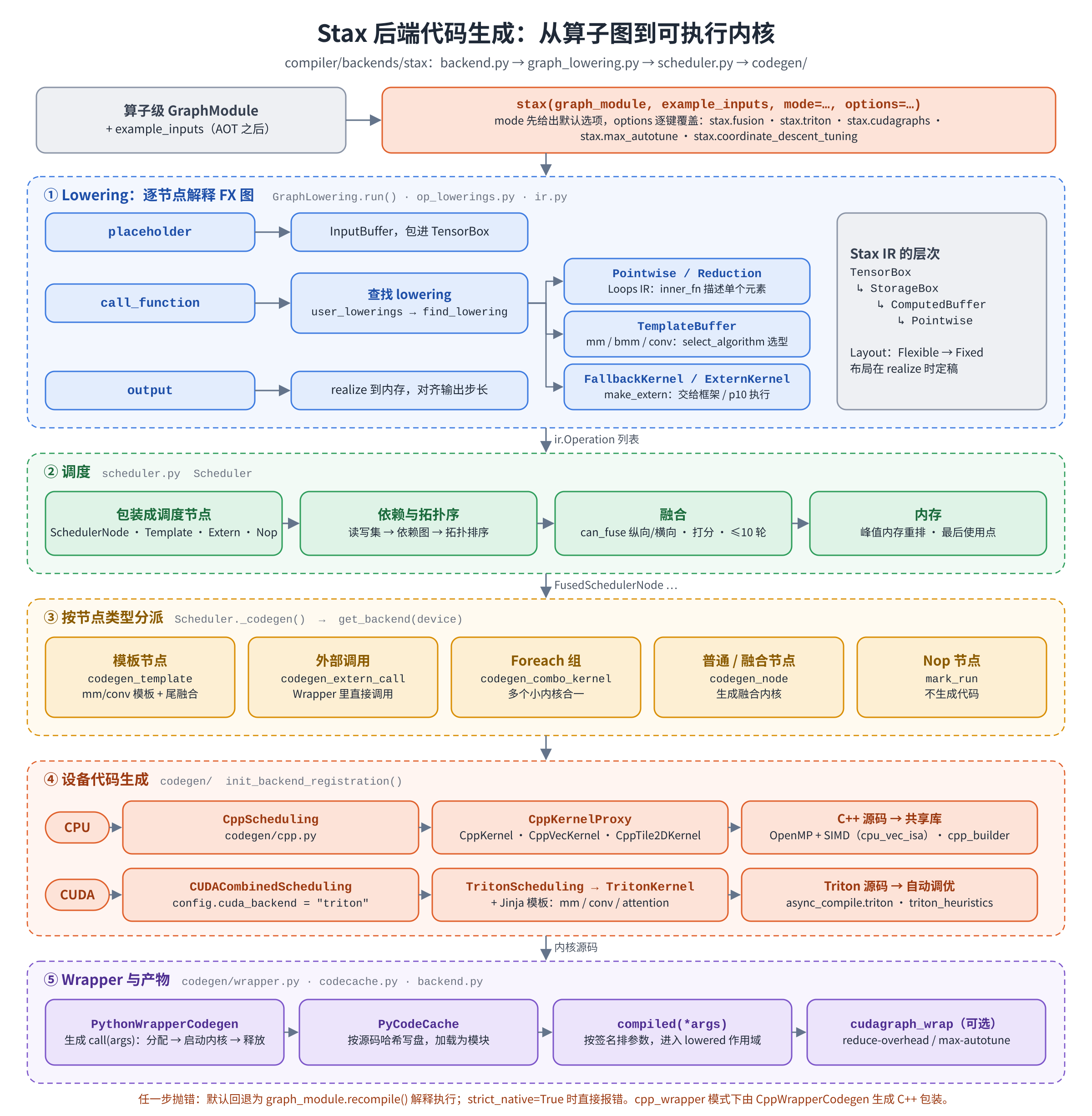
Figure 11.1 The flow of the Stax backend: lower to a loop-level intermediate representation, schedule and fuse, dispatch by node type, generate CPU or GPU kernels, and finally generate the wrapper function and store it in the code cache. The bottom of the figure records the fallback rules in case of failure.
The first call to cf(x, w) (Example 1.1, inference, CPU) passes through the following steps in order:
- The first-level dispatch entry has not been established yet; compute the specialization key $K$, and the specialization cache misses (Section 2.2、Section 2.4);
- Lift free tensors (there are none in this example), trace the function with run-time proxies, and obtain the graph of Listing 3.1; extract the guard-replay subgraph. This example has no data gates, so the subgraph is empty (第 Section 3);
- Normalization, constant folding, decomposition, common subexpression elimination, dead code elimination, and pointwise region marking run in turn to a fixed point (第 Section 4);
- The region is retraced at the dispatcher level, obtaining the operator-level graph of Listing 5.1; an inference region has no backward part 第 Section 5.1;
- Lowering: the compute functions of the four operators compose layer by layer into a single reduction node (Listing 6.2, Property 6.1);
- Scheduling: there is only one node, so there is nothing to fuse; a single 64-element output is allocated, consistent with the lower bound of Proposition 1.1 (第 Section 7);
- Code generation: generate the C++ kernel of Listing 1.1 and the wrapper function of Listing 8.1, compile and load them through the content-addressed cache (第 Section 8,Section 11.1、Section 11.2);
- The compiled artifact is registered in the specialization cache and recorded as the first-level entry; the computation runs and the result is returned.
Subsequent calls with the same tensors take a shortened path: the first-level entry checks the tensor object and its version counter, enters the call of the wrapper function, checks the shape and stride of the inputs, allocates the output, and calls the kernel.
The training case (Example 5.1) differs at step 4. The AOT layer traces a joint graph and partitions the forward graph from the backward graph by minimum cut (Section 5.3 to Section 5.5); the forward graph is compiled by steps 5 through 7, and the two are combined by a subclass of autograd.Function (Section 5.6). During forward execution $h$ is saved; the first call to backward compiles the backward graph by steps 5 through 7, and the resulting kernel recomputes erf from $h$ and multiplies it by the upstream gradient (Listings 5.3 and 9.3). On the GPU, step 7 generates a Triton kernel (第 Section 9); if CUDA Graphs is enabled, what step 8 registers is the wrapper object described in (Section 9.9).
12 Discussion
12.1 Comparison with PyTorch 2
Several class names in the Stax backend, such as GraphLowering, Scheduler, CachingAutotuner, and TritonKernel, together with the minimum-cut partitioner in the AOT layer, coincide with the corresponding parts of TorchInductor and AOTAutograd in PyTorch 2 [15]; the two are essentially identical in structure over lowering, scheduling, and code generation. A reader familiar with one of them can read the other at low cost. The main difference between the two lies in the front end.
TorchDynamo works at CPython’s frame-evaluation interface: it intercepts a function’s bytecode before the function runs, performs symbolic execution over the bytecode, and records tensor operations as a graph. When it meets a part it cannot record, such as a data-dependent branch or an untraceable external call, it performs a graph break: the function is cut into several segments, the capturable segments are compiled as graphs, and the bytecode between them is handed back to the interpreter. During symbolic execution it tracks modifications to Python objects (such as list appends and attribute assignment), and replays those modifications after graph execution.
TensorPlay’s front end instead executes the function for real at the Python level with proxy objects (第 Section 3). The two compare as follows:
- Data-dependent control flow. TorchDynamo breaks the graph there; TensorPlay selects a branch according to the sample data and records it as a data gate, confirming the branch on every call with a guard-replay subgraph (Section 3.4、Section 3.5). The former yields several smaller graphs; the latter yields one complete graph specialized to the data;
- Capture failure. TorchDynamo tolerates failure with a graph break; TensorPlay’s capture failure reports an error directly (Section 11.3), and a region is either compiled as a whole or not compiled at all;
- Python side effects. TorchDynamo replays recognizable side effects outside the graph; under TensorPlay’s tracing execution the function runs once, so pure Python side effects (such as printing logs or appending to a list) happen exactly once during capture, and subsequent calls execute the compiled artifact directly with no further side effects;
- The granularity of specialization. Both specialize on metadata such as shape and dtype, and both specialize Python scalars by value. TensorPlay additionally specializes on data gates, so the degree of specialization is higher and the cache may hold more versions (Example 3.2). For shapes, TorchDynamo automatically turns a dimension into a symbolic one when different sizes appear on it successively, whereas TensorPlay’s
compileprovides only a global switch: withdynamic=Trueit treats every dimension whose size is neither 0 nor 1 as symbolic from the start, using guards to distinguish different branches and layouts (Section 10.4); - The construction of guards. TensorPlay’s guards are a projection of the specialization key (Section 2.3), so every miss can locate the corresponding condition in the guard chain. Moreover, TensorPlay installs ahead of the guards one more C-level path that decides on object identity and version counter (Section 2.4), which has the lowest overhead for scenarios that repeatedly call with the same set of buffers.
12.2 Comparison with Abstract-Value-Tracing Systems
JAX [27] likewise constructs its computation graph by tracing, but the values passed in during tracing are abstract values carrying only shape and dtype. Abstract values have no concrete data, so Python’s if applied to a trace value raises an error directly, and data-dependent control flow must be rewritten into structured control-flow primitives such as lax.cond and lax.while_loop, with the compiler representing the branches inside the graph. TensorPlay’s run-time sampling sits between pure symbolic tracing and immediate execution: during tracing both symbolic and sample values are held, if can be evaluated on the sample value, and the cost is that the compiled result is valid only for inputs that take the same branch as the sample, which must be guarded by a data gate.
JAX’s jit caches compiled results by the abstract signature of the arguments and allows designated arguments to be specialized by value with static_argnums; TensorPlay specializes all Python scalars by value by default (Section 2.2), and when this must be avoided they should be wrapped as 0-dimensional tensors. Each default has its trade-off: specializing by value lets scalar constants participate in folding and simplification at compile time, but frequent changes of a scalar cause repeated compilation.
The symbolic_trace of torch.fx [5] is pure symbolic proxy tracing, identical in behavior to TensorPlay’s tracer with execute=False (Section 3.4). TensorPlay’s graph representation, including the six opcodes of Table 3.1, GraphModule, and the Python source it generates, is also consistent with torch.fx.
12.3 Comparison with Algorithm-Schedule Separation Compilers
Halide [16] proposes describing separately the algorithm (how each value is computed from other values) and the schedule (the order of computation, tiling, parallelization, and storage placement). The algorithm part writes each stage as a function from coordinates to values, which is the same representation as $\mathit{inner_fn}$ in Stax’s loop-level intermediate representation (Definition 6.1). The difference between the two lies in who supplies the schedule. Halide’s schedule is written explicitly by the programmer, or searched for by an auto-scheduler; TVM [28] inherits this separation and uses a cost-model-based search to find a schedule for an operator. Stax provides no schedule language, and scheduling decisions are made by a fixed set of heuristic rules: whether to materialize (Section 6.6), whether to split a reduction (Section 6.5), how to fuse (Section 7.3), how to tile and parallelize (Sections 8 and 9) and only the GPU launch configuration is chosen by measurement (Section 9.6). This approach has short compilation time and needs no offline search; the price is that in cases the heuristics do not cover, performance may fall below what a search could achieve.
Two further developments of the same idea are worth mentioning. Tiramisu [51] places the algorithm-schedule separation inside a polyhedral framework, where the schedule is expressed as an affine transformation (Section 7.7) and its legality is checked by criteria of the kind of Theorem 7.2; TACO [50] targets sparse tensor algebra and automatically generates loops over nonzero entries from the storage format and index expressions of the tensors, a direction not covered by Stax’s dense loop model. Ansor [49] builds on TVM to generate the search space of schedules automatically and guides the search with a learned cost model (Section 9.6).
TensorPlay additionally provides a TVM backend, which translates the captured graph into TVM’s compute description and lets TVM perform scheduling and code generation; it can serve as a control for the two sources of schedules.
12.4 Comparison with XLA and MLIR
XLA [35] is one of the earliest widely used tensor compilers and is also the default backend of JAX. Its input is HLO, a graph representation whose nodes are tensor operations and whose shapes are all static. Compared with Stax there are three points worth noting.
First, the unit of fusion. Fusion in XLA operates on the HLO graph, grouping mergeable operations into “fusion computations” and deciding legality by several fixed fusion kinds (loop fusion of pointwise chains, input fusion rooted at a reduction or a transpose, tail fusion of matrix multiplication, and so on), and each fusion computation then generates one kernel. Stax first completes pointwise fusion by function composition on the loop-level intermediate representation (Section 6.3), and then merges greedily between scheduling nodes by shared byte count 第 Section 7. Both face the same problem, the partitioning problem of Definition 7.3, and both use heuristic approximations; the difference is that Stax’s loop-level representation allows fusions such as “reduction followed by broadcast” to be decided directly from the index relation (Propositions 7.2 and 7.3) without enumerating case by case.
Second, shapes. HLO requires static shapes, and a dynamic dimension appears only in the form of a “shape with an upper bound”: allocation by the upper bound, carrying the actual size at run time. This is the limiting case of the same idea as the bucketing of Proposition 10.3, namely a single bucket. Stax’s symbolic shapes (第 Section 10) take a different route: shape classes are partitioned by guards, and each class generates shape-polymorphic code.
Third, layout. XLA has a dedicated layout assignment phase that chooses a dimension order for every tensor over the whole graph and inserts transposes where needed. Stax chooses layouts only for intermediate buffers (the flexible layout of Section 6.4); the layouts of inputs and outputs are determined by the caller.
MLIR [36] is not a compiler but a framework for building compilers. Its core concept is the dialect: each dialect defines a set of operations and types representing one abstraction level, for example linalg for structured tensor operations, affine for affine loops and indices, scf for general structured control flow, and gpu and nvvm for device code. Compilation is the progressive lowering between dialects, and each level can reuse analyses and transformations provided by the framework, such as dependence analysis and polyhedral transformations on the affine dialect (Section 7.2).
Setting Table 1.2 side by side with MLIR: Stax’s five layers of representation roughly correspond to the lowering chain “graph dialect → linalg → loop dialect → device dialect” in MLIR. The difference is that Stax’s layers are independently implemented Python data structures whose inter-layer interfaces are conventions rather than a type system, whereas MLIR’s layers share the infrastructure of a single intermediate representation, so a transformation written once applies to every dialect satisfying its interface. The former buys simplicity and the ability to debug directly in Python, which is the trade-off TensorPlay makes as a learning-oriented framework; the latter buys composability, at the price of a steeper learning curve and longer compiler construction time. Triton itself is built on top of MLIR, so the GPU kernels Stax generates ultimately also pass through MLIR’s lowering chain.
12.5 Design Principles
Taking the sections together, the Stax compiler stack has several designs that run through the whole chapter:
- Just-in-time compilation is program specialization, and a guard is a projection of the specialization key. The key and the guards come from the same data, and their consistency is guaranteed by construction rather than by testing (Section 2.1、Section 2.3);
- Data-dependent control flow is handled by specialization, the condition is extracted by reverse slicing, and the extraction must precede dead code elimination (Section 3.5);
- The algebraic simplifications in graph transformation are checked one by one against IEEE 754 semantics: identities that would change NaN, infinity, or the rounded result (such as $x \cdot 0 \Rightarrow 0$, reassociation) are never used; $x + 0 \Rightarrow x$, which differs only in the sign of zero, is the only inexact rewrite accepted. Termination of the rewrite system is guaranteed by a well-founded measure (Section 4.1、Section 4.2);
- Inference and training use the same operator-level graph, and the save-versus-recompute trade-off reduces to a minimum-cut problem (第 Section 5);
- A value is represented by default as a function and written into memory only when the cost model asks for it (Section 6.3、Section 6.6). Fusion is therefore the default behavior rather than an exception that must be proved pairwise;
- The splitting of reductions, vectorization, and online softmax are all grounded in the associativity of a semigroup (Section 6.5、Section 8.1、Section 9.5);
- The heuristic decisions on the compilation path (fusion, materialization, parallel depth, launch configuration) each correspond to an optimization problem that is generally NP-hard or can only be evaluated as a black box, and Stax gives approximate solutions by greedy or local search (Section 7.2、Section 9.6);
- Semantic preservation is the first promise, fallback guarantees it, and strict mode turns performance into a checkable contract as well 第 Section 11.3;
- The model precedes the measurement, and the measurement tests the model. Every optimization first yields a prediction in terms of memory bytes, an error bound, or the order of the cost, and is then checked against measurement; a speedup must be decomposed into a structural factor and an efficiency factor, and every discrepancy must be attributed 第 Section 13.
13 Models and Measurement
Most of the conclusions of the preceding sections come from models: the counting of memory traffic, the roofline, error bounds, and asymptotic orders of cost. A model yields falsifiable predictions, and the role of measurement is to test them. This section first establishes a statistical model of measurement itself 第 Section 13.1, then tests in turn the memory model of fusion gains 第 Section 13.2, the rounding-error model of summation 第 Section 13.3, and the amortization model of compilation overhead 第 Section 13.4, and finally discusses in what sense these tests are valid 第 Section 13.5.
13.1 A Statistical Model of Measurement
Experimental setup. The hardware is a 4-core Intel Xeon in the cloud (2.8 GHz, AVX-512, 32 KB L1d and 1 MB L2 per core, 33 MB shared L3); the software is the CPU build of the TensorPlay development branch, Python 3.13, with 4 threads. Each case is warmed up 3 times and then timed 15 times, taking the median. Compiled versions always use strict_native=True, guaranteeing that what is measured is a kernel generated by Stax rather than a fallback. All cases were measured completely in two separate rounds at different times, denoted A and B.
The reading of a timing is disturbed by other processes, interrupts, frequency scaling, and cache state. Interference can only slow one execution down, never speed it up, which gives the following model.
Definition 13.1 (Additive Nonnegative Noise) A reading of one timing is $T = t_0 + \varepsilon$, where $t_0$ is the undisturbed duration and $\varepsilon \ge 0$ is the delay introduced by interference. The $\varepsilon$ of the various readings are independent and identically distributed, and for every $\delta > 0$ we have $\Pr[\varepsilon < \delta] > 0$.
Proposition 13.1 Under Definition 13.1, the minimum $T_{(1)}$ of $n$ readings is a consistent estimator of $t_0$, and $\Pr[T_{(1)} - t_0 \ge \delta] = \Pr[\varepsilon \ge \delta]^n$.
Proof $T_{(1)} - t_0 \ge \delta$ holds if and only if every reading has $\varepsilon \ge \delta$, and independence gives the equality. By the assumption $\Pr[\varepsilon \ge \delta] < 1$, the right-hand side tends to 0 as $n \to \infty$. $\square$
The minimum estimates “what the machine can do”, and is therefore suited to estimating capability parameters such as bandwidth and arithmetic throughput; the median describes “what typically happens”, is insensitive to the few readings severely disturbed, and is therefore suited to comparing the typical duration of two ways of executing. The median also has an interval estimate that does not depend on the distribution.
Proposition 13.2 (Distribution-Free Confidence Interval for the Median) Let $X_1, \dots, X_n$ be independent and identically distributed from a continuous distribution with median $m$, and let $X_{(1)} \le \dots \le X_{(n)}$ be the order statistics. For $1 \le j < k \le n$,
$$\Pr\bigl[X_{(j)} \le m < X_{(k)}\bigr] = \sum_{i=j}^{k-1} \binom{n}{i} 2^{-n}.$$
Proof Let $K$ be the number of readings not exceeding $m$. Each reading does not exceed $m$ with probability $1/2$, so $K \sim \mathrm{Binomial}(n, 1/2)$. Now $X_{(j)} \le m$ if and only if $K \ge j$, and $m < X_{(k)}$ if and only if $K \le k - 1$, so the required probability is $\Pr[j \le K \le k-1]$. $\square$
Taking $n = 15$, $j = 4$, and $k = 12$ gives a coverage probability of $96.5%$: the 4th smallest and the 12th smallest readings form a 95% confidence interval for the median, independent of whatever distribution the readings follow. Proposition 13.2 requires the readings to be independent and identically distributed, and this assumption does not hold across different time periods: the load of the machine varies with time, and the difference between the medians of two rounds often exceeds the confidence interval of a single round. This section therefore compares two ways of executing only within one round, and lists the results of both rounds, taking the difference between the two rounds as the magnitude of the systematic error.
Machine parameters. The memory bandwidth $B$ is measured by a row-wise sum over a 64 MiB tensor. The two rounds together with three further repetitions give 7 medians, ranging from 1.36 ms to 3.18 ms, a difference of more than a factor of two. Following Proposition 13.1, capability parameters are taken as the minimum, so $B \approx 49.4$ GB/s; the arithmetic throughput $P$ is taken as the best result of a 2048-order float32 matrix multiplication, about 392 GFLOP/s. The ridge point $P/B \approx 7.9$ FLOP/byte, and the arithmetic intensity of the pointwise and reduction cases in this section is below 1, placing them on the sloping part of the roofline (Figure 1.1, left). The rate measured with copy_ is only 18.4 GB/s (counting one read and one write): when writing a line that is not in the cache, the processor must first read it in (write allocate), so the actual traffic exceeds the count. Models that count bytes therefore systematically underestimate the cost of writes.
13.2 Decomposing the Gains of Fusion
(Section 1.1) predicts the gains of fusion in terms of memory bytes. The following proposition says in what sense this prediction is exact, and what it misses.
Definition 13.2 (Model Byte Ratio and Effective Bandwidth) Let the numbers of main-memory bytes counted for immediate execution and for compiled execution by the method of (Section 1.1) be $b_e$ and $b_c$ respectively, and let the measured durations be $T_e$ and $T_c$. Call $\rho = b_e / b_c$ the model byte ratio, and call $\beta_e = b_e / T_e$ and $\beta_c = b_c / T_c$ the effective bandwidth of the two ways of executing.
Proposition 13.3 (Decomposition of the Speedup) The speedup $S = T_e / T_c$ satisfies
$$S = \rho \cdot \frac{\beta_c}{\beta_e}.$$In particular, if the two ways of executing attain the same fraction of the bandwidth ceiling, then $S = \rho$; and $S > \rho$ if and only if the compiled kernel is closer to the bandwidth ceiling than the kernel of immediate execution.
Proof $S = \dfrac{b_e / \beta_e}{b_c / \beta_c} = \dfrac{b_e}{b_c} \cdot \dfrac{\beta_c}{\beta_e}$. $\square$
Proposition 13.3 is an identity; its value is that it splits the speedup into two factors of quite different character. The factor $\rho$ is determined by the structure of the graph and is the gain brought by the decisions about fusion and materialization (Sections 6 and 7) it can be computed before compilation, and by Proposition 1.1 it is bounded above. The factor $\beta_c / \beta_e$ is the ratio of kernel quality, which depends on vectorization, parallel partitioning, and the memory access pattern (第 Section 8); the byte model makes no assertion about it at all. An optimization that claims a speedup should say how much of it comes from $\rho$ and how much from $\beta_c / \beta_e$.
Table 13.1 lists six cases. The inputs are float32 tensors of size $8192 \times 2048$ (64 MiB, far larger than L3), and a softmax row is $16384 \times 1000$. The two numbers in each cell come from rounds A and B respectively.
Table 13.1 Duration and effective bandwidth of immediate execution and compiled execution (CPU, 4 threads, median, rounds A / B)
| Case | $\rho$ | Eager (ms) | Compiled (ms) | $S$ | $\beta_e$ (GB/s) | $\beta_c$ (GB/s) |
|---|---|---|---|---|---|---|
Example 1.1: (relu(x + w) * 2).sum(-1) | 4.00 | 16.6 / 15.6 | 3.38 / 3.94 | 4.91 / 3.95 | 32.3 / 34.4 | 39.7 / 34.0 |
Example 7.1: x / x.sum(-1, keepdim=True) | 1.50 | 5.80 / 5.90 | 4.65 / 4.97 | 1.25 / 1.19 | 34.7 / 34.1 | 28.9 / 27.0 |
| softmax (five hand-written operators, Section 9.5) | 4.00 | 23.8 / 17.7 | 7.68 / 7.85 | 3.09 / 2.26 | 22.1 / 29.6 | 17.1 / 16.7 |
softmax (library operator F.softmax) | 1.00 | 7.94 / 7.85 | 9.82 / 9.46 | 0.81 / 0.83 | 16.5 / 16.7 | 13.4 / 13.9 |
Example 7.2: exp followed by sum and amax | 2.00 | 14.0 / 14.6 | 7.34 / 8.53 | 1.90 / 1.72 | 28.8 / 27.5 | 27.5 / 23.6 |
| LayerNorm → GELU → multiply by 0.5 | — | 16.0 / 17.6 | 10.7 / 11.1 | 1.50 / 1.58 | — | — |
The $\rho$ of Example 7.2 is computed according to the materialization decisions on CPU (Section 6.6): immediate execution computes exp twice, reading and writing each time, and each result is then read once by a reduction, for $6N$ elements in total; after compilation exp is computed once and written into a buffer, and the two reductions are fused into a single pass of reads, for $3N$.
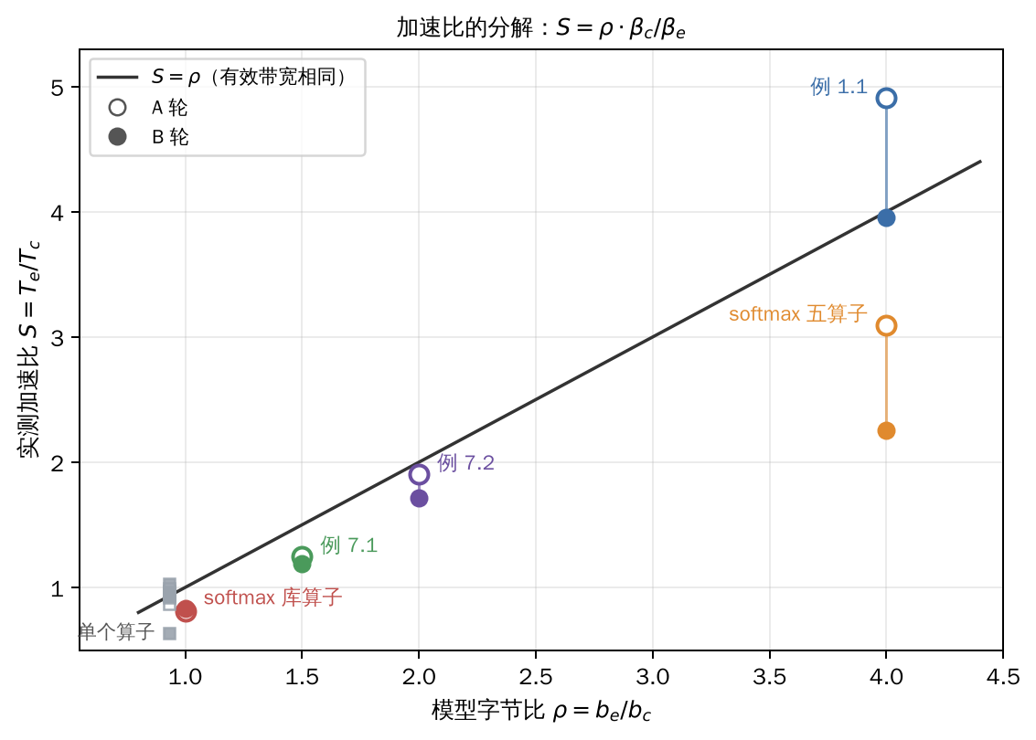
Figure 13.1 The measured speedup $S$ against the model byte ratio $\rho$. The solid line is $S = \rho$, that is, equal effective bandwidth for the two ways of executing; points below the line indicate that the compiled kernel is further from the bandwidth ceiling. Hollow and filled markers are rounds A and B respectively; the points at $\rho = 1$ are the library softmax of Table 13.1 and the five single operators of Table 13.2 (squares, shifted slightly to the left so as not to overlap).
The structural factor determines the magnitude. In Figure 13.1, as $\rho$ varies from 1 to 4, $S$ rises from about 0.8 to about 4, and the two are distributed roughly along $S = \rho$. The byte model predicts the magnitude and the ordering of the speedup, which is exactly what (Section 1.1) needs: to decide whether a fusion is worth doing, one looks at how many bytes can be saved.
The efficiency factor determines the deviation. Example 1.1 gives $S = 4.91 > \rho$ in round A because the fused kernel reaches 80% of $B$ in effective bandwidth while the two pointwise kernels of immediate execution reach only 65%; in round B both are around 70%, and $S = 3.95 \approx \rho$. The five-operator softmax also has $\rho = 4$, yet $S$ is only 3.09 and 2.26, and the reason lies in the factor $\beta_c / \beta_e$: the fused kernel reaches only 35% of $B$. For each row it first computes the maximum, then the exponential sum, and finally the division; there are data dependences between the three passes, so a row cannot be pipelined; the row length 1000 is not a multiple of the vector width 16, so the end of every row carries a masked tail. These are all kernel-quality problems discussed in 第 Section 8, and the byte model does not count them. For the library softmax $\rho = 1$, the compiler cannot reduce the bytes, so $S$ is left with only the efficiency factor; since the compiled kernel is slightly slower than the hand-written library kernel, $S \approx 0.82$.
Table 13.2 gives another set of examples with $\rho = 1$: a single operator has no intermediate tensor to eliminate.
Table 13.2 Duration of single operators ($8192 \times 2048$, ms, rounds A / B)
| Operator | Eager | Compiled | $S$ |
|---|---|---|---|
exp | 4.66 / 4.54 | 4.81 / 4.71 | 0.97 / 0.96 |
x + 1 | 3.79 / 3.90 | 4.04 / 4.18 | 0.94 / 0.93 |
relu | 4.12 / 3.91 | 4.24 / 4.24 | 0.97 / 0.92 |
row-wise sum | 3.15 / 1.36 | 3.18 / 2.14 | 0.99 / 0.63 |
row-wise amax | 2.03 / 3.23 | 2.34 / 3.15 | 0.87 / 1.03 |
Eight of the ten ratios fall between 0.87 and 1.03: when $\rho = 1$, compilation offers no gain, and the single kernel generated is of comparable quality to the library kernel, a few percent slower. Row-wise sum differs by more than a factor of two between the two rounds (3.15 ms and 1.36 ms), while amax, which has the same memory traffic in the same period, moves in the opposite direction; this is exactly the inter-period systematic error described in (Section 13.1), and the median of a single round cannot hide it.
13.3 A Statistical Model of Rounding Error
(Section 6.5) gave the worst-case error bound for summation. For Example 1.1, each row is a sum of 2048 nonnegative numbers drawn from the same distribution, with a row sum of about 2300. The bound for sequential summation is $(n-1) u \sum |a_i| \approx 0.28$, 16-way segmented summation is about $0.020$, and tree summation is about $1.5 \times 10^{-3}$, while in both rounds the maximum measured difference between the compiled result and the eager result is $4.9 \times 10^{-4}$. The worst-case bound requires every rounding to attain its maximum with the same sign; actual rounding errors have both signs and partially cancel each other. The following model describes the typical case [18].
Theorem 13.1 (A Statistical Model of Summation Error) Let $\hat s_1 = a_1$ and $\hat s_k = (\hat s_{k-1} + a_k)(1 + \delta_k)$, $k = 2, \dots, n$, where the $\delta_k$ are mutually independent and independent of the data, $\mathbb E[\delta_k] = 0$, and $\mathrm{Var}[\delta_k] = \sigma_\delta^2 \le u^2$. Writing the partial sums $s_k = \sum_{i \le k} a_i$, the error $E = \hat s_n - s_n$ under a first-order approximation satisfies
$$E \approx \sum_{k=2}^{n} \delta_k s_k, \qquad \mathbb E[E] = 0, \qquad \mathrm{Var}[E] = \sigma_\delta^2 \sum_{k=2}^{n} s_k^2.$$If the rounding errors are uniformly distributed on $[-u, u]$, then $\sigma_\delta^2 = u^2/3$.
Proof Induction on $n$ gives $\hat s_n = \sum_{i} a_i \prod_{k = \max(i,2)}^{n} (1 + \delta_k)$. Expanding the products and dropping terms of degree two and above in $\delta$ gives $\hat s_n - s_n \approx \sum_{k=2}^{n} \delta_k \sum_{i \le k} a_i = \sum_{k=2}^{n} \delta_k s_k$. The zero mean and the variance formula follow from the independence and zero mean of the $\delta_k$; the variance of the uniform distribution is $u^2/3$. $\square$
Corollary 13.1 Let the $a_i$ be independent and identically distributed with mean $\mu$ and variance $\sigma^2$, let the summation be split into $W$ ways ($W$ a power of two), each way accumulating $n/W$ numbers sequentially, and let the $W$ partial sums finally be merged in a tree. Then
$$\mathrm{Var}[E] \approx \frac{u^2}{3}\Bigl(\underbrace{\frac{n^3 \mu^2}{3 W^2} + \frac{n^2 \sigma^2}{2 W}}_{\text{per-way accumulation}} + \underbrace{2 n^2 \mu^2 + n \sigma^2 \log_2 W}_{\text{tree merge}}\Bigr).$$When the mean is nonzero and $n \gg W^2$, the standard deviation of the error grows as $n^{3/2}$; when the mean is zero it grows as $n$.
Proof For each way the $k$-th partial sum satisfies $\mathbb E[s_k^2] = k^2 \mu^2 + k \sigma^2$. Summing over $k = 1, \dots, n/W$ gives $\frac{(n/W)^3}{3} \mu^2 + \frac{(n/W)^2}{2} \sigma^2$ (keeping the highest orders), and multiplying by the number of ways $W$ gives the first part. At the $\ell$-th level of the tree merge ($\ell = 1, \dots, \log_2 W$) there are $W/2^\ell$ additions, each with a result that is the sum of $2^\ell n/W$ numbers and has second moment $(2^\ell n \mu / W)^2 + 2^\ell n \sigma^2 / W$; summing level by level gives $\frac{n^2\mu^2}{W}(2W - 2) + n\sigma^2\log_2 W \approx 2n^2\mu^2 + n\sigma^2 \log_2 W$. Substituting both parts into Theorem 13.1 gives the claim. $\square$
Whether the merge term can be neglected depends on the relation between $n$ and $W$: when the mean is nonzero its ratio to the leading term is about $6W^2/n$, so it is a lower-order term only when $n \gg W^2$; when the mean is zero the ratio is about $2W\log_2 W / n$, which is usually negligible.
Apply Corollary 13.1 to two cases, taking $u = 2^{-24}$ and $W = 16$ (the number of float32 lanes of AVX-512).
Example 1.1: $a_i = 2,\mathrm{relu}(z)$, $z \sim \mathcal N(0, 2)$, $\mu = 2\sqrt{2}/\sqrt{2\pi} \approx 1.13$. Here $6W^2/n \approx 0.75$, so the merge term cannot be neglected; taking both parts, the standard deviation of the error per row is about $1.7 \times 10^{-4}$. Assume that the compiled result and the eager result each have independent, identically distributed errors (both accumulate in 16 ways); the standard deviation of their difference is multiplied by $\sqrt 2$, giving about $2.4 \times 10^{-4}$, and the maximum over 8192 rows is about 3.9 standard deviations, i.e. $9.5 \times 10^{-4}$. The measurement is $4.9 \times 10^{-4}$, exactly 2 times the spacing between adjacent float32 numbers at the magnitude of the row sum ($2^{11}$ to $2^{12}$): the error itself is quantization. Prediction and measurement are of the same order, with the prediction about 2 times larger, consistent with the case of Example 7.1 below.
Example 7.1: $a_i \sim \mathcal N(0, 1)$, $\mu = 0$, and the standard deviation of the error of a row sum is about $u n / \sqrt{6W} \approx 1.25 \times 10^{-5}$. Normalization passes the error in the row sum directly to each output, so the relative error is about $|E| / |s|$ and is largest on the row whose sum has the smallest absolute value. The smallest row sums in the two rounds are 0.0152 and 0.0050, the predicted maximum relative errors (including $\sqrt 2$) are $1.2 \times 10^{-3}$ and $3.5 \times 10^{-3}$, and the measurements are $6.3 \times 10^{-4}$ and $1.4 \times 10^{-3}$. Both the order of magnitude and the direction of variation with the smallest row sum agree with the prediction; the measurement is about 2 times smaller, which is consistent with the kernel unrolling the reduction loop into several groups of vector accumulators (an effective $W$ greater than 16), since the standard deviation is proportional to $1/\sqrt W$.
Example 7.1 also shows the role of the condition number. The relative condition number of normalization is $\kappa = \sum|x_i| / |\sum x_i|$, and the worst row in round B is about $3 \times 10^5$. On another set of random inputs of the kind used in Table 13.1, the maximum absolute error is 0.16 and 2.9 in rounds A and B respectively; this looks like a bug but is in fact the amplification of ordinary rounding error by ill-conditioned inputs. (Section 11.4) says that the criterion for “consistent” must leave room for tolerance; here is a concrete example: the tolerance must be set relative to the condition number of the problem, and a fixed absolute tolerance will misjudge ill-conditioned inputs as compilation errors.
The errors of the remaining cases are below $10^{-6}$. In the training case (Example 5.1, $x \in \mathbb R^{4096\times1024}$, $W \in \mathbb R^{1024\times1024}$), the relative error between the compiled and the eager gradients is $1.8 \times 10^{-7}$, about $3u$.
13.4 Amortizing Compilation Overhead
Let the one-time cost of compiling one specialized version be $C$, and let the duration of each subsequent call be $t_c$ under compilation and $t_e$ under immediate execution.
Proposition 13.4 (Break-Even Point) If $t_e > t_c$, then the total compilation time after $m$ calls does not exceed that of immediate execution if and only if
$$m \ge m^* = \frac{C}{t_e - t_c}.$$
Proof Rearranging $C + m t_c \le m t_e$ gives the result. $\square$
For Example 1.1 on $8192 \times 2048$, the first call with a cold compilation takes 5.6 to 5.9 s, each call saves 11.6 to 13.2 ms, and $m^* \approx 420$ to $510$. The cost $C$ can be decomposed further: on release 1.1.0, a cold compilation of Example 1.1 in a new process with $64 \times 128$ inputs takes 5.2 to 5.5 s; starting another new process with the same cache directory brings the first call down to about 1.2 s. The difference of about 4 s is the time of the external C++ compiler, which is saved by the content-addressed cache of (Section 11.1); the remaining about 1.2 s is capture, graph transformation, lowering, scheduling, and code generation, all of which every new process must redo. On a cache hit, $m^*$ drops to about 100.
Proposition 13.4 concerns a single specialized version. If a workload produces $K$ distinct specialization keys, the total one-time cost is $KC$, and the size of $K$ is determined by the specialization strategy of 第 Section 2and 第 Section 10.
Proposition 13.5 (Expected Number of Specialized Versions) Suppose the shapes of the various calls are drawn independently from a distribution $p$, that is, the probability of shape $s$ is $p_s$. When specializing on the concrete shape, the number $K_m$ of specialized versions produced by $m$ calls satisfies
$$\mathbb E[K_m] = \sum_s \bigl(1 - (1 - p_s)^m\bigr).$$If instead one buckets by powers of two as in Proposition 10.3, with sizes ranging over $[m_0, M_0]$, then for any $m$ there is $K_m \le \lceil \log_2 M_0 \rceil - \lfloor \log_2 m_0 \rfloor + 1$.
Proof $K_m = \sum_s \mathbf 1[\text{shape } s \text{ appears at least once}]$; by linearity of expectation, $\mathbb E[K_m] = \sum_s \Pr[s \text{ appears at least once}] = \sum_s (1 - (1 - p_s)^m)$. With bucketing each bucket produces at most one version, and by Proposition 10.3 the number of buckets does not exceed the right-hand side. $\square$
For example, when the sequence length is uniformly distributed between 1 and 512, specializing on the concrete shape gives an expected number of versions after 1000 calls of about $512(1 - (511/512)^{1000}) \approx 440$, and amortization is almost impossible; after bucketing there are at most 10 versions; with dynamic shapes 第 Section 10there is only one version as long as no guard fails.
Call overhead. The cost $C$ is measured in seconds, whereas the fixed overhead of each call is measured in microseconds. For x * 2 + 1 on 8 elements, immediate execution (two operators) takes 3.6 μs per call; the compiled version, called repeatedly with the same tensor, takes 12.0 to 12.7 μs, going through the first-level entry of (Section 2.4) and checking only object identity and version counter; when a new tensor is passed each time it takes 22.0 to 22.6 μs, since the signature must be computed and the specialization cache looked up.
Proposition 13.6 (Minimum Size for Fusion to Pay Off) Suppose a chain of $k$ pointwise operators acts on $N$ float32 elements, each operator reading one tensor and writing one tensor. Let the fixed overhead per operator under immediate execution be $\tau_e$, the fixed overhead per call after compilation be $\tau_c$, and the effective bandwidth of both ways of executing be the same $\beta$. Then compiled execution is faster if and only if
$$N > N^* = \frac{(\tau_c - k \tau_e)\,\beta}{8 (k - 1)}.$$
Proof Immediate execution takes $k\tau_e + 8kN/\beta$, and compiled execution takes $\tau_c + 8N/\beta$. Their difference is $8(k-1)N/\beta - (\tau_c - k\tau_e)$, and rearranging gives the result. $\square$
Taking $k = 2$, $\tau_e = 1.8$ μs, and $\beta = B$: for repeated calls with the same tensor $N^* \approx 5 \times 10^4$, and for a new tensor passed each time $N^* \approx 1.1 \times 10^5$, that is, a few hundred KB. Small tensors stay resident in the cache, so the actual bandwidth exceeds $B$ and $N^*$ would only be larger. The compiler is therefore suited to regions whose computational work greatly exceeds the call overhead; for programs composed of many small operators, they should be placed into the same compiled region so that $k$ grows while $\tau_c$ is paid only once.
13.5 The Validity of the Tests
The extent to which a test can support a model depends on its validity. Following the conventions of experimental methodology, it can be examined in three aspects; the common pitfalls and norms for reporting performance in parallel computing are in [37].
Construct validity asks whether the quantity measured is really the quantity the model speaks about. The $b$ of the byte model is main-memory traffic, while the actual traffic of a kernel also includes write allocate (Section 13.1) and the re-reads of cache misses; the inputs of the cases are far larger than L3 precisely so that main-memory traffic dominates. strict_native=True guarantees that what is measured is the generated kernel rather than the result of falling back to immediate execution.
Internal validity asks whether the observed difference is genuinely caused by the factor under study. Timing the two ways of executing back to back within the same round reduces the influence of inter-period drift, but does not eliminate it entirely; alternating timing (rotating between the two ways for each reading) is a better design; but the differences between the two rounds (Tables 13.1 and 13.2) show that the median of a single round is not enough to support conclusions at the 10% level. Only effects that agree in direction across the two rounds and are much larger than the difference between the rounds — for example, the difference between $\rho = 4$ and $\rho = 1$ — can be regarded as established.
External validity asks whether the conclusions generalize. The data come only from one shared cloud host, with no fixed processor frequency; there is no GPU, so the conclusions about the GPU in 第 Section 9have not been measured; the cases are all single small functions and do not cover a complete model. In the training case both ways of executing take between 650 and 730 ms per step, far exceeding the sum of the forward and backward kernels of the two matrix multiplications and the GELU (under 80 ms); the duration is dominated by the fixed overhead of the automatic differentiation engine and lies outside the applicability of the byte model, so this section reports no speedup for it.
Within these limits, the measurement supports the three models of this chapter: the gains of fusion are determined in magnitude by the model byte ratio, and the deviations are explained by the ratio of effective bandwidths (Proposition 13.3); the rounding error is far smaller than the worst-case bound, and both its order of magnitude and the direction in which it varies with the condition number are given by the statistical model (Corollary 13.1); the one-time cost of compilation is measured in seconds and the call overhead in microseconds, and the two determine where compilation pays off through Propositions 13.4 and 13.6.
Chapter Summary
This chapter has taken the Stax compiler stack of TensorPlay as its object and has discussed the various stages of compiling tensor programs into efficient kernels, together with the theory that supports each stage.
Just-in-time compilation is program specialization. Tracing the function on sample inputs yields a graph that is valid only for inputs with the same specialization key (Proposition 2.1); the specialization key consists of the signature, the shape, and the data gates, and the guards are its projection, so that every recompilation can supply a condition that does not hold (Corollary 2.1). Data-dependent control flow is likewise handled by specialization: computations on which a branch condition depends are extracted by reverse slicing into a guard-replay subgraph, and the extraction must precede dead code elimination (Proposition 3.1, Corollary 3.1).
Graph transformation is a rewrite system whose termination is guaranteed by a well-founded measure (Proposition 4.1). Floating-point numbers do not satisfy the algebraic laws of the reals, so algebraic simplification must be checked one by one against IEEE 754 semantics: identities that would change NaN, infinity, or the rounded result are not used, and $x + 0 \Rightarrow x$, which only changes the sign of zero, is the sole accepted exception. Common subexpression elimination is value numbering, dead code elimination is backward reachability, and both can be done in linear time. Operator-level decomposition expands only those operators that are not in the base of the backend, and its termination likewise follows from a well-founded depth (Proposition 4.3); functionalization eliminates in-place modification and view aliasing by means of a scatter inverse, making the graph a pure function (Proposition 4.4), and in-place reuse at the scheduling stage then reclaims the storage.
A training region obtains a joint graph by reverse-mode automatic differentiation, at a cost no more than a constant multiple of the forward pass (Theorem 5.1, with the constant no more than 5 for the usual elementary functions). Which values to save in the forward pass and which to recompute in the backward pass reduces to a minimum cut on the rematerialization network (Proposition 5.1), solved in polynomial time by the max-flow min-cut theorem; under a storage constraint, binomial checkpointing inverts a chain with logarithmic storage and recomputation factors (Theorem 5.4). Forward mode propagates tangent vectors with dual numbers and is suited to the case of many outputs and few inputs; the compilation path currently supports only first-order reverse mode, and second-order differentiation raises an explicit error 第 Section 5.7.
Lowering represents every value as a function from indices to values, and the fusion of pointwise operations is precisely function composition (Property 6.1); a view is an affine transformation of the index space (Proposition 6.2); the splitting and parallelization of reductions are grounded in the associativity of a semigroup, and in the floating-point case the price is a different rounding-error bound. The denotational semantics of the core language turn these claims into theorems: inlining and materialization, and common subexpression elimination, preserve semantics bit by bit (Theorems 6.1 and 6.2), while the rearrangement of reductions preserves only real-number semantics (Theorem 6.3). Whether a value is written into memory is decided by comparing the recomputation cost with the memory-access cost. Loop bodies are normalized, and adjacent loops are merged when the stride conditions are satisfied (Proposition 6.3); range analysis over interval domains is sound (Proposition 6.4), and on that basis provably redundant bounds checks are omitted and 32-bit indices are chosen.
Scheduling searches for fusion plans on the dependence graph. Fusion presupposes the compatibility of iteration spaces (Definition 7.2), and the correctness of vertical fusion is guaranteed by agreement between the read and write indices (Proposition 7.2). Optimal fusion is NP-hard (Theorem 7.1); Stax adopts a greedy algorithm whose primary gain is shared bytes, and uses Proposition 7.1 to maintain acyclicity. The legality of interchange, skewing, and tiling of multiply nested loops is decided by distance vectors (Theorems 7.2 and 7.3), and the existence of a one-dimensional affine schedule can be reduced to linear programming by Farkas’ lemma (Proposition 7.5). Buffer reuse is a storage allocation problem on an interval graph, while the topological order minimizing peak memory is NP-complete (Proposition 7.4, by a reduction from path width); Stax picks the best among several heuristic orders.
Code generation prints the same loop-level description as a program on CPU or GPU. On the CPU, the legality of vectorization comes from the independence of iterations or from the associativity of reductions (Proposition 8.1), tiling makes cache lines fully utilized, and the choice of parallel depth balances load balance against fixed overhead. On the GPU, Little’s law gives the concurrency needed to hide memory latency; the single-pass form of softmax relies on a semigroup on $(m, d)$ pairs (Proposition 9.1); the choice of launch configuration is a black-box optimization, for which coordinate descent gives a local optimum (Proposition 9.2) and random search gives a quantile guarantee (Proposition 9.3); and the tiling of matrix multiplication asymptotically attains the I/O lower bound proved by the Loomis–Whitney inequality (Theorem 9.1).
Dynamic shapes are a coarsening of the shape component of the specialization key, and their soundness requires that the compiled artifact be valid over the entire equivalence class (Proposition 10.1). Symbolic shapes record the judgments about sizes made during tracing as shape guards; a guard is either implied by the declared range or becomes a run-time assertion, and every size-dependent decision in the backend must either hold over the whole range or be restricted by a guard. Stax’s CPU and GPU kernels share the same symbolic lowering; multiple artifacts under the same key are distinguished by their own guards, and during training both the forward and the backward artifacts can be reused across sizes.
Reuse of compilation results is the memoization of a pure function, and content addressing lets the cache dispense with invalidation (Proposition 11.1); the completion time of parallel compilation is given by the bound on list scheduling (Proposition 11.2). The constraint running through the whole chapter is semantic preservation: every transformation must preserve the semantics of the program, fallback guarantees this, and strict mode turns performance into a checkable contract as well.
(Section 9.10) discussed attention: the triple of online softmax allows attention to be tiled like a reduction, block masks lift sparsity to the granularity of blocks, and score_mod and mask_mod are embedded into the template in the form of subgraphs. 第 Section 13checked the models of the whole chapter by measurement: the speedup equals the product of the model byte ratio and the ratio of the effective bandwidths (Proposition 13.3), the former determining the magnitude and the latter explaining the deviation; the statistical model of summation error gives a prediction two to three orders of magnitude below the worst-case bound and in agreement with measurement (Theorem 13.1); and the break-even point of compilation and the minimum size for fusion to pay off are given by two simple cost models (Propositions 13.4 and 13.6).
This chapter did not touch custom operators, the overlap of computation and communication in distributed training, or convolution templates; readers may consult the source index in Appendix A on their own.
Exercises
Difficulty markers: ★ directly applies a conclusion of the main text; ★★ requires a full derivation or proof; ★★★ an open or research-type problem, which may require consulting the literature. Exercises with hints or solutions are in Appendix C.
★ Suppose the shapes of $x$ and $w$ in Example 1.1 are $n\times128$ and the dtype is float32. (1) Compute the numbers of memory bytes and the arithmetic intensity for immediate execution and for fully fused execution, as functions of $n$. (2) Prove that fused execution attains the lower bound of Proposition 1.1. (3) If
sum(-1)is removed, what does the lower bound become? How does the proportion saved by fusion change?★ For the
g(x, k) = x * kof Example 2.1, (1) state on which inputs the compiled artifact violates the conclusion of Proposition 2.1 if the value of $k$ is not in the specialization key. (2) Give a rewrite that makes $k$ part of the dynamic part, and state what constant folding loses after the rewrite.★ Construct an example in which the guards and the specialization key are maintained separately, the keys already differ, and all the guards still hold, and explain what error then occurs. Then point out at which step the proof of Corollary 2.1 uses the fact that “the guards are a projection of the key”.
★★ (1) Prove that the time complexity of Algorithm 3.1 is $O(|V| + |E|)$. (2) Suppose the guard-replay subgraph of Example 3.2 is extracted after dead code elimination; give the result of the second call, and explain why this error cannot be detected by the guards of (Section 2.3).
★ Let $x$ be an arbitrary float32 value (including $\pm 0$, $\pm\infty$, NaN, and subnormals). For each of the following, decide whether the rewrite holds exactly under IEEE 754 semantics, and give a counterexample where it does not: (1) $x \cdot 1 \Rightarrow x$; (2) $x + 0 \Rightarrow x$; (3) $x - 0 \Rightarrow x$; (4) $x \cdot 0 \Rightarrow 0$; (5) $x - x \Rightarrow 0$; (6) $x / 2 \Rightarrow x \cdot 0.5$; (7) $x / 3 \Rightarrow x \cdot (1/3)$.
★★ Give a set of rewrite rules that makes the fixed-point iteration of (Section 4.1) fail to terminate, and indicate which condition of Proposition 4.1 it violates. If $a + b \Rightarrow b + a$ and constant folding are added to the rule set at the same time, how should the measure $\mu$ be chosen to guarantee termination?
★★ Suppose the operator-level decomposition table contains the rules $o_1 \Rightarrow o_2 + o_3$ and $o_2 \Rightarrow o_1 \cdot c$, with $o_1, o_2 \notin \mathcal B$. (1) Explain why the depth in Proposition 4.3 is not well-defined, and what happens when the decomposition recurses. (2) If $o_2$ is added to the base of the backend, is the depth well-defined?
★★ For
y[0].add_(1)in Example 4.4, (1) write the definitions ofselectandselect_scatterand verify the two conditions of Proposition 4.4. (2) If it is changed toy.t()[0].add_(1), which nodes should the graph after functionalization contain? (3) Explain why common subexpression elimination done before functionalization may go wrong.★★ In Example 5.1, replace gelu with relu, and assume that the backward of relu reads the output of relu. (1) Reconstruct the rematerialization network according to Definition 5.2 and find the minimum cut. (2) How do the saved values differ from Table 5.1? How many more bytes must the forward pass write?
★★ Suppose a value $v$ in the forward pass is the result of a reduction and is read by the backward pass, that is, $v \in U \cap B$ (case 3 in 第 Section 5.4). (1) Prove from Definition 5.1 that $v$ belongs to every feasible save set. (2) Verify the same conclusion in the network of Definition 5.2: explain why every cut of finite capacity must cut $v_{\mathrm{in}} \to v_{\mathrm{out}}$.
★★ (1) Suppose the layout of $x$ is shape $(4, 6)$ with strides $(6, 1)$; find the layout of
x.t(), and use the conditions of (Section 6.4) to decide whetherx.t().reshape(24)can be expressed as a set of strides. (2) Prove: for any layout, slicing then transposing and transposing then slicing give the same $(t’, o’)$.★ Suppose the loop body has three nested loops with extents $(4, 8, 16)$, and the indices of the two memory accesses are $128 i_0 + 16 i_1 + i_2$ and $i_0 + 4 i_1 + 32 i_2$. According to Proposition 6.3, decide which adjacent loops can be merged, and explain whether reordering the loop nest first could make the merge possible.
★★ (1) According to Definition 6.4, find the intervals of $(3i + 5) \bmod 128$ and $\lfloor i / 4 \rfloor - 1$ ($i \in [0, 511]$), and decide which of them can dispense with a bounds check. (2) Construct an index expression whose run-time values always lie in $[0, 127]$ but for which interval analysis cannot prove this. Does this contradict Proposition 6.4?
★★ Suppose a segment of elements has count, mean, and second central moment $(n, \mu, M_2)$. (1) Write the merge operation for two segments and prove that it satisfies associativity and commutativity [17]. (2) Compare the numerical stability of this merge with “computing $\sum x$ and $\sum x^2$ separately and then subtracting”, and explain why the latter fails when $\mu^2 \gg \mathrm{Var}(x)$.
★★ For the triple $(m, \ell, \mathbf a)$ of (Section 9.10): (1) Prove in detail that the merge operation satisfies associativity and commutativity, and state what the identity element is. (2) Suppose the forward pass saves $\mathrm{LSE}i = m_i + \log \ell_i$; prove that in the backward pass $P{ij} = \exp(S_{ij} - \mathrm{LSE}i)$, and explain why saving only $m_i$ or only $\ell_i$ is not enough. (3) From $dP = dO, V^{\mathsf T}$ and the derivative of softmax, write the expression for $dS$ and show that it needs only one block of $P$ and $D_i = \sum_j dO{ij} O_{ij}$.
★ Let $n = 2^{20}$. According to (Section 6.5), compute the error bound coefficients for sequential summation, for segmented summation with $k = 16$, for segmented summation with $k = 1024$, and for tree summation, and explain why the number $W$ of vector accumulators should not be too small.
★★ (1) For the graph $a \to c \to b$, $a \to b$, verify that merging $a$ and $b$ creates a cycle. (2) Construct a dependence graph and a gain function such that the greedy result of Algorithm 7.1 has a cost strictly greater than that of the optimal fusion plan.
★★ Suppose all intermediate buffers have the same size. Prove: the greedy algorithm that sorts by the left endpoint of the lifetime and each time allocates the lowest-numbered free slot uses a number of slots equal to $\max_\tau |L(\tau)|$, and hence attains the lower bound of Definition 7.5. Give an example showing that this conclusion fails when the buffer sizes differ.
★ Construct two nodes $a \to b$ whose iteration spaces are compatible and which share data, but where $b$ reads the output of $a$ at index $w(i+1)$. Explain what value the fusion in the order of Proposition 7.2 would read, and why the scheduler rejects this fusion.
★ Suppose the dependence graph consists of two chains $a \to c$ and $b \to d$, the outputs of $a$ and $b$ each occupy 4 units and are released after their unique user executes; $c$ and $d$ are outputs of the graph, each occupying 1 unit and not released. Enumerate all topological orders, compute the peak memory of each according to Definition 7.5, and explain which order the minimum-peak-first rule of (Section 7.5) selects.
★ (1) According to Algorithm 8.1, find the parallel depth of the three nested loops $4\times4096\times16$ when $P = 8$ and $m = 512$; what if $P = 64$? (2) In $q \in [2P, 3P]$, when does $\lceil q/P \rceil / (q/P)$ attain its maximum? What is the maximum?
★ Suppose global memory latency is $\lambda$ and bandwidth is $B$, each SM holds $w$ warps, and each thread issues a 16-byte read per instruction. By Little’s law, find the minimum number of reads that must be in flight per thread to saturate the bandwidth. Compute it with the numbers of (Section 9.1) and $w = 32$ and 132 SMs, and explain what this result implies for the choice of block size.
★ Do a row-wise softmax on a float32 tensor of shape $n\times L$. (1) Find the ratio of the memory bytes of the fused kernel of (Section 9.5) to those of five separate kernels. (2) When $L$ exceeds the limit of a persistent reduction, how many times does each of the two-pass form and the online form have to read the input?
★★ Construct a cost function $t$ on $\Pi = {1, 2, 4, 8}^2$ such that Algorithm 9.2, starting from some initial point, stops at a configuration that is not globally optimal.
★ For a float32 matrix multiplication with $m = n = k = 4096$, suppose the on-chip storage of each program instance holds at most $S = 48 \times 1024$ elements, and take $B_M = B_N = T$ and $B_K = 32$. (1) Find the largest power of two $T$ satisfying the capacity constraint. (2) Find the main-memory traffic and the arithmetic intensity in that case, and compare them with $I_{\max}$. (3) For $\mathrm{relu}(AB + \mathbf b)$, find the proportion of the matrix-multiplication traffic saved by tail fusion.
★ Suppose a region consists of $n$ kernels, each with device execution time $t$. From the model of (Section 9.9), find an expression for the speedup of CUDA Graphs in terms of $n$, $t$, $t_{\mathrm{launch}}$, and $t_{\mathrm{graph}}$, and find its upper bound.
★ (Section 9.9) points out that the output replayed by CUDA Graphs lies in a memory pool dedicated to the graph. Explain why the contents of the list are incorrect in a training loop that appends the output to a list at every step once CUDA Graphs is enabled, and explain how this relates to the specialization described in Proposition 2.1.
★★ Suppose a function contains the branch
if x.shape[0] % 8 == 0:, is specialized with a sample whose dimension 0 is 64, and declares that dimension as $n \in [1, 1024]$. (1) Write the resulting shape guard, and state which case of (Section 10.2) it belongs to. (2) If insteadcompileon the concrete shape is used and it is called successively with dimension 0 equal to $1, 2, \dots, 64$, how many specialized versions are produced? And how many after bucketing as in Proposition 10.3?★ Suppose a float32 tensor of shape $(n, 128)$ is summed row-wise, with $n \in [1, 2^{24}]$. (1) Find the maximum value of the index expression and decide whether 32-bit indices can be used. (2) If $n$ is declared without an upper bound, what two approaches can the backend take? What is the cost of each? (3) Explain why the number of segments in splitting a reduction can only be chosen according to a hint value, and what this implies for correctness and for performance.
★★ (1) Prove the birthday bound in Proposition 11.1. (2) Construct a situation in which $\mathrm{build}$ is not a pure function of $(s, a)$, so that the cache returns a stale artifact, and explain how to extend $a$ to rule this out.
★★ Prove that the upper bound of Proposition 11.2 can be improved to $\frac1P \sum_i c_i + (1 - \frac1P) \max_i c_i$, and construct a set of tasks showing that this bound is tight.
★★★ Compare run-time proxy tracing (TensorPlay), bytecode-level capture (TorchDynamo), and abstract-value tracing (JAX) in four aspects: data-dependent control flow, Python side effects, degree of specialization, and the handling of compilation failure; and explain these differences from the viewpoint of program specialization.
★★ Suppose the $i$-th iteration of $a$ writes $B[i]$ and the $i$-th iteration of $b$ reads $B[i-1]$ ($i \ge 1$). (1) Find the dependence distance, and according to Proposition 7.3 decide whether sequential fusion and parallel fusion are legal. (2) What if it reads $B[i+1]$ instead? (3) For the case of (1), explain how it can be rewritten on the GPU so that the fused kernel is still correct (hint: have each program instance compute one extra element). What is the cost?
★★ In Table 13.2, the speedups of the single compiled operators mostly fall between 0.87 and 1.03. (1) According to Proposition 13.3, what does $S$ equal when $\rho = 1$? (2) Row-wise
sumgives $S = 0.63$ in round B. Under the model of Definition 13.1, explain why this single number is not enough to prove that the compiled kernel is slower, and design an experiment that can decide the question (hint: alternate the timing, and apply Proposition 13.2 to the difference between the readings of the two ways). (3) Suppose write allocate makes the actual traffic of a write 1.5 times the count. Recompute $\rho$ for Example 1.1 and compare it with $S = 4.91$ from round A of Table 13.1.★ For Proposition 9.4: (1) Suppose $g_m = g_n = 16$ and $W = 24$; find the number of input blocks read simultaneously for row-major numbering and for $G = 4$ and $G = 8$ respectively. (2) How should the conclusion of the proposition be modified when $G$ does not divide $W$? (3) What determines the number $W$ of simultaneously running instances? Which configuration parameters of (Section 9.6) is it related to?
★ Suppose $N = 8192$, $d = 128$, on-chip storage $M = 100 \times 1024$ elements, float16. (1) By Theorem 9.2, estimate the ratio of the main-memory accesses of per-operator attention to those of blocked attention. (2) If the backward pass is also considered, the per-operator implementation must save $P$ while the blocked implementation saves only LSE; find the ratio of the bytes saved by the two.
★ Sliding-window attention allows only the positions with $|q - k| \le w$ to participate. Suppose the sequence length is $N$, the block size is $B$, and $w$ is an integer multiple of $B$. (1) Find the numbers of full blocks, partial blocks, and empty blocks. (2) Compared with the causal mask, what proportion of computation does block masking save? (3) If $w$ is not an integer multiple of $B$, how does the number of partial blocks change?
★★ Let $f: \mathbb R^{1000} \to \mathbb R^{10}$, and suppose the cost of computing $f$ is $W$. (1) Compute the full Jacobian matrix in forward mode and in reverse mode respectively; what is the cost of each? (2) What if only one $J v$ and one $u^{\mathsf T} J$ are needed? (3) Explain why compiled regions do not support second-order derivatives, and what the AOT layer would have to do additionally in order to support them.
★★ Suppose
n = x.nonzero().shape[0]is followed by the branchif n > 0:. (1) Explain why this test cannot be evaluated on the sample and recorded the way the shape guards of (Section 10.2) can. (2) If the user knows for certain thatxhas at least one nonzero element, how should the program be rewritten so that it can be compiled? (3) How does this relate to Proposition 10.4?★ (1) The nominal arithmetic throughput of FP8 tensor cores is about 2 times that of BF16. By the method of (Section 9.8), find the minimum order at which an FP8 square matrix multiplication on H100 becomes compute-bound. (2) Taking $B_M = B_N = 128$, $B_K = 128$, and FP8, find the on-chip storage occupied by each pipeline stage, and the upper bound of
num_stagesunder 228 KB of shared memory.★★ For Proposition 13.2: (1) Verify that the coverage probability is $96.5%$ for $n = 15$, $j = 4$, and $k = 12$. (2) Using the minimum and maximum $[X_{(1)}, X_{(n)}]$ as the confidence interval for the median, find the smallest $n$ giving a coverage probability of at least 99%. (3) 第 Section 13.1points out that readings are no longer identically distributed across different periods. Suppose a total of $r$ rounds are measured, each with $n$ readings, and the medians $m_1, \dots, m_r$ of the rounds are independent and identically distributed; give a confidence interval for the “overall median”, and explain how it differs from applying Proposition 13.2 to the $rn$ readings pooled together.
★★★ For Theorem 13.1: (1) Under the same model, find the error variance of pairwise tree summation ($n = 2^L$), for the two cases $\mu = 0$ and $\mu \ne 0$, and compare its order of growth in $n$ with that of the $W$-way segmented summation of Corollary 13.1. (2) Taking $n = 2048$, $\mu = 0$, and $\sigma = 1$, compare the error standard deviations of sequential summation, 16-way segmented summation, and tree summation. (3) The first-order error term of Kahan compensated summation is independent of $n$. Explain at which step the derivation of Theorem 13.1 no longer applies, and why compensated summation cannot be used together with an arbitrary reassociation (Section 6.5).
★★ For Proposition 13.5: (1) Suppose the size $s \in {1, \dots, 512}$ follows a truncated Zipf distribution $p_s \propto 1/s$; compute $\mathbb E[K_{1000}]$ numerically and compare it with the about 440 of the uniform distribution. (2) Prove that $\mathbb E[K_m]$ is a concave function of $m$, and that $\mathbb E[K_m] \le \min(m, |{s : p_s > 0}|)$. (3) Bucketing rounds the size $s$ up to the smallest power of two not less than it, so the amount of computation per call at most doubles. Suppose the compilation cost is $C$ and a single call of size $s$ takes $\alpha s$. Write the expected total duration over $m$ calls for specialization on the concrete shape and for bucketing, and give the conditions under which bucketing is better.
★★ For Proposition 13.6: (1) Generalize to the case where the $i$-th operator reads $r_i$ tensors and writes one tensor, and find $N^$. (2) If $N$ is small enough that all the data resides in L2 and the effective bandwidth is $\beta_2 > B$, how does $N^$ change? For the machine of this section, how does the upper bound on $N$ given by the L2 capacity compare with $N^$? (3) From the data of (Section 13.4), estimate $N^$ for a chain of 5 pointwise operators, and explain why compilation becomes increasingly advantageous as $k$ grows.
★★★ (Research problem) Theorem 7.1 allows an arbitrary given set of forbidden pairs. (1) Prove: if the iteration spaces of all nodes are pairwise compatible and no illegal dependence distance exists, then a minimum-cost fusion plan can be found in polynomial time. (2) The forbidden pairs of Stax are determined by the equivalence classes of iteration spaces (Definition 7.2) and by dependence distances (Proposition 7.3). Prove or refute: on this restricted problem class, minimum-cost fusion is still NP-hard (hint: consider a dependence graph in which two iteration spaces appear alternately and are joined by a reduction, and consult [55]).
★★ For Theorem 5.1: (1) For a program containing only additions and multiplications, what is the largest factor by which the total cost of reverse mode can exceed that of the forward pass? (2) Suppose $f(x) = \prod_{i=1}^n x_i$ is computed with $n - 1$ multiplications. Write the backward pass, verify that it computes all $n$ partial derivatives with $O(n)$ operations, and give the cost if each partial derivative is computed independently. (3) Explain why forward mode needs $\Theta(nW)$ operations for the same gradient, and how this relates to Proposition 5.2.
★★ For Theorem 9.1: (1) Take the parameters of Exercise 25 ($m = n = k = 4096$, $S = 48 \times 1024$), compute the numerical value of the lower bound, and compare it with the tiled traffic of Exercise 25. By roughly how many factors do the two differ? Where does the gap come from? (2) Suppose there are $P$ processors, each with a fast memory of capacity $S$, and all products are evenly distributed. Prove that some processor transfers no fewer than $\dfrac{mnk}{2\sqrt3,P\sqrt S} - S$ times. (3) Explain why the theorem does not apply to Strassen’s algorithm, and how the I/O lower bound for Strassen’s algorithm should be stated.
★★ For the reduction of Proposition 7.4: (1) Take $H$ to be the path $P_4$ on 4 vertices and the cycle $C_4$ on 4 vertices, compute $\mathrm{vs}(H)$ for each, construct $D$, and find the minimum of the peak over all topological orders, verifying that it falls in the interval given by the proof. (2) If the dependence graph is a tree (each node has at most one user), explain that the peak-minimizing topological order can be found in polynomial time (hint: Sethi–Ullman numbering).
★★ For (Section 6.9): (1) Prove $\mathrm{view}{\pi_1}(\mathrm{view}{\pi_2}(e)) \equiv \mathrm{view}_{\pi_2 \circ \pi_1}(e)$ and compare it with the affine composition of Proposition 6.2. (2) Add to the core language a random-number operation $\mathrm{rand}(\sigma)$ parameterized by an explicit state $\sigma$, whose semantics also returns the new state. Explain under what conditions Theorem 6.2 (1) holds for it. (3) Give a program in which deleting the unused bindings changes its observable behavior, and use it to write the definition of the refinement relation.
★★ For (Section 7.7): suppose the distance vectors of a doubly nested loop are $(1, 0)$, $(0, 1)$, and $(1, -1)$. (1) By Theorem 7.2, decide whether loop interchange is legal; is the loop band fully permutable? (2) Find a unimodular skew transformation that makes the transformed loop band fully permutable, so that it can be tiled. (3) Following the idea of Lemma 7.1, find a one-dimensional affine schedule $\theta(i, j) = c_1 i + c_2 j$ such that every distance vector satisfies $c \cdot \delta \ge 1$; explain which iterations can execute in parallel under a one-dimensional schedule.
★★ For Theorem 5.4: (1) Compute $\beta(3, 3)$ and write a complete reversal order for a chain of length 6 with $s = 3$ and $t = 2$. (2) For chain length $l = 1000$, find the minimum number $s$ of slots required for $t = 2, 3, 4$ respectively. (3) Compare the result of (2) with the uniform partitioning of Theorem 5.3 (at most two computations per step, $2\sqrt l$ of storage).
★★ For Proposition 9.3: (1) Taking $q = \delta = 0.01$, find the required number $N$ of samples. (2) Construct a cost function such that coordinate descent (Algorithm 9.2), starting from some initial point, stops within the slowest 10%, while random search avoids it with high probability. (3) How does the conclusion of Proposition 9.3 change in practice when there is noise? Design a scheme that allocates measurement counts by successive halving [54], and estimate the total number of measurements it requires.
Programming Labs
The following labs take TensorPlay’s source code as their object; each takes roughly 4 to 8 hours. Labs 1 and 2 require only the installed package; labs 3 through 5 require an editable install from source (pip install -e . --no-build-isolation, see the repository’s CLAUDE.md); lab 6 requires a CUDA device. The deliverable of each lab consists of code, data, and an analysis of at most one page, and the analysis must set the measurements against the models of this chapter.
Lab 1 Roofline and Attribution. (1) On your own machine, measure the memory bandwidth and the matrix-multiplication arithmetic throughput, and plot the measured roofline 第 Section 13.1. (2) Reproduce Tables 13.1 and 13.2, and plot each case on the roofline. (3) For each case, first write out the model-predicted speedup by the method of 第 Section 1.1, then compare it with the measurement; for those differing by more than 20%, find the cause by means of a single-operator baseline or by changing the problem size. (4) Increase the input size step by step from $2^{10}$ elements to $2^{26}$ elements, plot the curve of speedup against size, and explain the changes of the curve near the L2 and L3 capacities. Appendix B gives the starter code.
Lab 2 Reading the Generated Code. Set the environment variable TP_CACHE_DIR to an empty directory, and compile Example 1.1, Example 7.1, Example 7.2, and a function of your own. The generated wrapper functions are saved as .py files in subdirectories of that directory named by content hash (Section 11.1), with the C++ kernels embedded in them as strings. (1) For each function, locate the wrapper function, mark every allocation, every kernel call, and every free, and compare them against the lifetime analysis of (Section 7.5). (2) For Example 7.2, verify the conclusion that exp is materialized on CPU but not on GPU (Section 6.6), and point out the evidence in the generated code. (3) Pass x and x.t() in turn for the same square matrix; two wrapper functions appear in the cache directory. Compare the strides in their assert_size_stride and the index expressions in the kernels, and explain why they differ.
Lab 3 Adding a Lowering Rule. In tensorplay/compiler/backends/stax/op_lowerings.py, find an operator that currently executes as a fallback kernel but is essentially pointwise (you may first use TP_STAX_LOWER_DEBUG=1 together with strict_native=True to find the operators that cannot be lowered). (1) Write a lowering rule for it using register_lowering and the pointwise helper of (Section 6.2), with a compute function that uses only the ops interface. (2) Write tests for it covering broadcasting, non-contiguous inputs, zero-element tensors, and special values ($\pm 0$, $\pm\infty$, NaN), comparing pointwise against immediate execution. (3) Measure its duration before and after fusion with the adjacent pointwise operation, and compare with the prediction of Proposition 1.1.
Lab 4 Changing the Score for Fusion. The gain function for fusion lives in score_fusion in tensorplay/compiler/backends/stax/choices.py, and the legality check is can_fuse in the same file (Section 7.3). (1) Construct a function that makes Algorithm 7.1 choose between two legal fusions (the construction of Exercise 17 can serve as a starting point). (2) Modify the lexicographic order of the gain function, for example raising the distance $\delta$ above the byte count, and observe the changes in the fusion result and the peak memory. (3) Turn off horizontal fusion and measure the change in the duration of Example 7.2. (4) Write a report explaining which scoring you think is better, and over what range your evidence holds.
Lab 5 Guards for Dynamic Shapes. Referring to the counting backend in test/stax/test_stax_symbolic_shapes.py, count the number of artifacts generated by tp.compile(fn, dynamic=True). (1) Reproduce the two conclusions of Example 10.4: the shape branch generates 2 artifacts, and the sizes 0, 1, and the general size generate 3 artifacts. (2) The check function returned by shape_guards.build_input_guard carries a source attribute; print it and explain one by one which assumption each of its conditions comes from (Section 10.4). (3) Construct a function whose number of artifacts grows linearly with the number of kinds of input size, and then rewrite it into a constant number using the method of (Section 10.4).
Lab 6 Variants of Attention (requires CUDA). (1) Implement sliding-window attention with omni_attention (Exercise 37), check the sparsity of the block mask with BlockMask.sparsity(), and compare it with your calculation in Exercise 37. (2) For $N = 1024, 2048, \dots, 16384$, measure the duration and the peak memory of the hand-written per-operator attention, of F.scaled_dot_product_attention, and of omni_attention, and explain the way in which the peak memory grows with $N$ by Theorem 9.2. (3) Add to score_mod a bias that depends on a learnable tensor, verify that the backward pass differentiates it, and compare the duration with and without score_mod.
Previous: Part Four GPU Code Generation and Dynamic Shapes | Table of Contents | Next: Part Six References and Appendix