Stax (4): GPU Codegen and Dynamic Shapes

Previous: Part Three　Scheduling, Fusion and CPU Code Generation　｜　Table of Contents　｜　Next: Part Five　Caching, Discussion, Models and Measurements; Summary and Exercises

Bibliography numbers [n] in the text refer to Part Six; section numbers, theorem numbers and exercise numbers are numbered uniformly across the whole chapter, and cross-section references remain valid.

9 GPU Code Generation

On CUDA devices, template nodes such as matrix multiplication and convolution are handed to the template code generators (see Section 9.8), while the remaining pointwise, reduction and fused nodes are generated as Triton [23] kernels. This section first introduces the execution model of the GPU and the programming model of Triton, and then discusses in turn pointwise kernels, the three forms of reduction kernels, multi-reduction fusion, the choice of launch configuration, matrix multiplication, and CUDA Graphs.

9.1 Execution Model and Programming Model

A GPU consists of a number of streaming multiprocessors (SMs). Each SM holds multiple thread blocks resident simultaneously, and threads are grouped 32 at a time into warps; the threads of the same warp execute the same instruction at the same instant. The guiding idea of GPU design is to hide latency with concurrency: a single global memory access has a latency of several hundred clock cycles, and during that time the SM switches to executing other ready warps.

This idea can be stated quantitatively with Little’s law. Let the latency of global memory be $\lambda$ and its bandwidth be $B$; for the bandwidth to saturate, the number of bytes in flight must reach

at any instant. Estimating with $\lambda \approx 600\ \mathrm{ns}$ and $B = 3.35\ \mathrm{TB/s}$, roughly 2 MB of memory traffic must be in flight, which spread over 132 SMs gives about 15 KB per SM. The more warps are resident and the more independent memory accesses each thread issues, the easier this degree of concurrency is reached. The number of warps resident on an SM at the same time is limited by registers and shared memory: the more registers each thread uses, the fewer warps can be resident. This is the root of the trade-off between block size and warp count in Section 9.4 and Section 9.6.

The efficiency of memory access also depends on coalescing: if the 32 threads of a warp access a contiguous and aligned range of addresses, the hardware merges them into a few memory transactions; if the addresses are scattered, each thread needs its own transaction, and the effective bandwidth drops by a corresponding factor. This is analogous to the cache-line analysis on the CPU in Section 8.2.

CUDA C takes the individual thread as its programming unit, and the programmer has to deal explicitly with warps, shared memory and coalesced access. Triton takes the thread block as its programming unit: a kernel is launched as a number of program instances, each of which processes one tile of data, and the parallelism within a block and the coalescing of its memory accesses are the responsibility of the Triton compiler.

Definition 9.1 (Program Instances and Blocks)　A Triton kernel is launched with a grid, every point of which is a program instance whose coordinates are obtained with tl.program_id(axis). Computation inside an instance is expressed in units of blocks: tl.arange(0, BLOCK) produces an index vector of length BLOCK, tl.load(ptr + offsets, mask) reads according to the vector indices, and positions where mask is false are not accessed; tl.store works the same way. A block size must be a compile-time constant (tl.constexpr) and a power of two.

Under this model, Stax’s loop-level intermediate representation maps fairly directly onto kernels: each dimension of the iteration range corresponds to one index vector, each ops call in inner_fn corresponds to one block-level operation, and out-of-range positions are masked off. The block size is not decided by code generation; it is left as a kernel parameter to be chosen empirically (Section 9.6).

9.2 The Structure of a Kernel

Listing 9.1 is the Triton kernel generated for Example 1.1 on a CUDA device, that is, the complete form of Listing 1.2 in Section 1.1(with all index-variable definitions retained), so that the two can be compared paragraph by paragraph.

Listing 9.1　The Triton kernel of Example 1.1 (import statements and decorator arguments omitted)

@triton_heuristics.persistent_reduction(size_hints={'x': 64, 'r0_': 128}, ...)
@triton.jit
def triton_per_fused_0(in_ptr0, in_ptr1, out_ptr0, xnumel, r0_numel, XBLOCK : tl.constexpr):
    xnumel = 64
    r0_numel = 128
    R0_BLOCK: tl.constexpr = 128
    rnumel = r0_numel
    RBLOCK: tl.constexpr = R0_BLOCK
    xoffset = tl.program_id(0) * XBLOCK
    xindex = xoffset + tl.arange(0, XBLOCK)[:, None]
    xmask = xindex < xnumel
    r0_index = tl.arange(0, R0_BLOCK)[None, :]
    r0_offset = 0
    r0_mask = tl.full([R0_BLOCK], True, tl.int1)[None, :]
    roffset = r0_offset
    rindex = r0_index
    r0_1 = r0_index
    x0 = xindex
    tmp0 = tl.load(in_ptr0 + (r0_1 + 128*x0), xmask, eviction_policy='evict_first', other=0.0)
    tmp1 = tl.load(in_ptr1 + (r0_1 + 128*x0), xmask, eviction_policy='evict_first', other=0.0)
    tmp2 = (tmp0 + tmp1)
    tmp3 = tl.full([1, 1], 0, tl.int32)
    tmp4 = tl.maximum(tmp3, tmp2, tl.PropagateNan.ALL)
    tmp5 = tl.full([1, 1], 2.0, tl.float32)
    tmp6 = (tmp4 * tmp5)
    tmp7 = tl.broadcast_to(tmp6, [XBLOCK, R0_BLOCK])
    tmp9 = tl.where(xmask, tmp7, 0)
    tmp10 = tl.sum(tmp9, 1)[:, None].to(tl.float32)
    tl.store(out_ptr0 + (x0), tmp10, xmask)

The kernel consists of four parts.

(1) Signature and constants. The parameters are, in order, the input pointers, the output pointer, the number of elements in each dimension, and the block sizes. When the shape is statically known, the element counts are rewritten as constants at the beginning of the function body (xnumel = 64), so that the Triton compiler can simplify the masks and the address computations accordingly.

(2) Indices and masks. The pointwise dimension x and the reduction dimension r0_ each correspond to one index vector. xindex has shape [XBLOCK, 1] and r0_index has shape [1, R0_BLOCK]; after broadcasting, the two form a two-dimensional XBLOCK × R0_BLOCK block: each program instance processes XBLOCK rows, all 128 elements of every row. xmask masks off the positions beyond the 64 rows; the reduction dimension has length 128, exactly equal to the block size, so the code generator determines that its mask is always true and writes it directly as tl.full(..., True, ...).

(3) Computation. tmp0 through tmp6 correspond one-to-one to the individual ops calls of inner_fn in Listing 6.2. ops.load becomes a masked tl.load, and the index expression 128*i0 + r0_0 becomes the address offset verbatim; ops.relu becomes tl.maximum(0, x, tl.PropagateNan.ALL), where PropagateNan.ALL guarantees that the output is also NaN when the input is NaN, consistent with the semantics of eager execution. eviction_policy='evict_first' tells the hardware that this data is read only once and may therefore be evicted from the L2 cache first.

(4) Reduction and write-back. Positions masked off are first set with tl.where to 0, the identity element of the reduction, then summed along dimension 1 with tl.sum, and finally the XBLOCK results are written back with tl.store.

Compared with the CPU kernel of Listing 1.1, both come from the same loop-level intermediate representation and differ only in how they are printed: the CPU kernel traverses the two dimensions with explicit loops, whereas the Triton kernel processes one XBLOCK × 128 block at a time with block-level vector operations, the loop being replaced by the grid and the parallelism within the block.

9.3 Pointwise Kernels and Two-Dimensional Tiling

A pointwise kernel has no reduction dimension, only one or more pointwise dimensions. Listing 9.2 is the kernel for Example 6.1 (x.t() + y).

Listing 9.2　The Triton kernel of Example 6.1 (import statements and decorator arguments omitted)

@triton_heuristics.pointwise(size_hints={'y': 256, 'x': 512}, tile_hint=TileHint.DEFAULT, ...)
@triton.jit
def triton_poi_fused_0(in_ptr0, in_ptr1, out_ptr0, ynumel, xnumel, YBLOCK : tl.constexpr, XBLOCK : tl.constexpr):
    ynumel = 256
    xnumel = 512
    yoffset = tl.program_id(1) * YBLOCK
    yindex = yoffset + tl.arange(0, YBLOCK)[:, None]
    ymask = yindex < ynumel
    xoffset = tl.program_id(0) * XBLOCK
    xindex = xoffset + tl.arange(0, XBLOCK)[None, :]
    xmask = xindex < xnumel
    x1 = xindex
    y0 = yindex
    tmp0 = tl.load(in_ptr0 + (256*x1 + y0), xmask & ymask)
    tmp1 = tl.load(in_ptr1 + (x1 + 512*y0), xmask & ymask)
    tmp2 = (tmp0 + tmp1)
    tl.store(out_ptr0 + (x1 + 512*y0), tmp2, xmask & ymask)

The indices of the two inputs are 256*x1 + y0 and x1 + 512*y0 respectively: the former is contiguous along y, the latter along x. With one-dimensional tiling, that is, treating the $256\times512$ outputs as a single vector of length 131072 and cutting it into blocks, the $x^{\mathsf T}$ elements read by adjacent threads lie 256 floats apart in memory, so the accesses cannot be coalesced. Two-dimensional tiling works with YBLOCK × XBLOCK rectangles: within a block, elements adjacent along y are contiguous for the first input, and elements adjacent along x are contiguous for the second input and for the output, so the Triton compiler can reorder the accesses within the block and give coalesced accesses on both sides. The grid is therefore two-dimensional, with program_id(1) corresponding to y and program_id(0) to x, and the grid type in the metadata is Grid2D.

Whether to use two-dimensional tiling is decided by the tiling selection of the SIMD layer: each candidate split of the dimensions is scored by how many bytes of memory access it can coalesce, and the scheme with the highest score whose number of dimensions does not exceed the limit is chosen (at most three dimensions by default). Both inputs of Example 1.1 are contiguous along the reduction dimension, so a single dimension suffices; the two inputs of Example 6.1 are contiguous in different directions, so two dimensions are chosen.

Listing 9.3 is the pointwise kernel for the GELU backward pass in Example 5.1, which can be compared against the CPU version of Listing 5.3 (Listing 5.4 in Section 5.5is an excerpt of it).

Listing 9.3　The backward pointwise kernel of Example 5.1 (GPU, import statements and decorator arguments omitted)

@triton_heuristics.pointwise(size_hints={'x': 2048}, ...)
@triton.jit
def triton_poi_fused_0(in_ptr0, in_ptr1, out_ptr0, xnumel, XBLOCK : tl.constexpr):
    xnumel = 2048
    xoffset = tl.program_id(0) * XBLOCK
    xindex = xoffset + tl.arange(0, XBLOCK)[:]
    xmask = xindex < xnumel
    x0 = xindex
    tmp0 = tl.load(in_ptr0 + (0))
    tmp1 = tl.broadcast_to(tmp0, [XBLOCK])
    tmp2 = tl.load(in_ptr1 + (x0), xmask)
    tmp3 = tl.full([1], 0.7071067811865476, tl.float32)
    tmp4 = (tmp2 * tmp3)
    tmp5 = libdevice.erf(tmp4)
    tmp6 = tl.full([1], 1.0, tl.float32)
    tmp7 = (tmp6 + tmp5)
    tmp8 = tl.full([1], 0.5, tl.float32)
    tmp9 = (tmp8 * tmp7)
    tmp10 = (tmp2 * tmp2)
    tmp11 = tl.full([1], -0.5, tl.float32)
    tmp12 = (tmp11 * tmp10)
    tmp13 = libdevice.exp(tmp12)
    tmp14 = tl.full([1], 0.3989422804014327, tl.float32)
    tmp15 = (tmp14 * tmp13)
    tmp16 = (tmp2 * tmp15)
    tmp17 = (tmp9 + tmp16)
    tmp18 = (tmp1 * tmp17)
    tl.store(out_ptr0 + (x0), tmp18, xmask)

in_ptr0 is the upstream gradient. Because the forward output loss is a scalar, the upstream gradient has only one element; the kernel reads it with tl.load(in_ptr0 + (0)) and broadcasts it over the whole block. in_ptr1 is the $h$ saved by the forward pass. tmp9 is $\Phi(h)$, tmp15 is $\varphi(h)$, and tmp17 is $\Phi(h) + h\varphi(h)$, i.e., $\mathrm{GELU}’(h)$, corresponding term by term to the derivation in Section 5.5. The erf and exp calls use device functions from libdevice.

9.4 The Three Forms of Reduction Kernels

Reduction kernels take one of three forms, depending on the length of the reduction dimension.

(1) Persistent reduction. If the reduction dimension is short enough, one program instance can read an entire row into registers and complete the reduction in a single pass, with no loop and no accumulator that has to be carried across iterations. Listing 9.1 is of this form, and the kernel-name prefix is per. Whether persistent reduction is used is decided by the following rules: when the reduction runs along a contiguous dimension (INNER), the length may be at most 1024; in other cases the length may be at most 64, and the lower and upper bounds of the length must be the same power of two. The block size R0_BLOCK is taken as the smallest power of two that is not less than the reduction length, and the excess is masked off.

(2) Looped reduction. When the reduction dimension is long, each program instance loops along the reduction dimension with stride R0_BLOCK, maintaining an XBLOCK × R0_BLOCK accumulator in registers, and reduces along dimension 1 into one value per row after the loop ends. The kernel-name prefix is red.

(3) Reduction splitting. When there are too few outputs, the lowering phase has already split the reduction into two levels (Section 6.5), and code generation accordingly produces two kernels.

Listing 9.4 gives the two kernels of Example 6.2, the first being a looped reduction and the second a persistent reduction.

Listing 9.4　The two Triton kernels of Example 6.2 (import statements and decorator arguments omitted)

@triton_heuristics.reduction(size_hints={'x': 128, 'r0_': 8192}, reduction_hint=ReductionHint.INNER, ...)
@triton.jit
def triton_red_fused_0(in_ptr0, out_ptr0, xnumel, r0_numel, XBLOCK : tl.constexpr, R0_BLOCK : tl.constexpr):
    xnumel = 128
    r0_numel = 8192
    rnumel = r0_numel
    RBLOCK: tl.constexpr = R0_BLOCK
    xoffset = tl.program_id(0) * XBLOCK
    xindex = xoffset + tl.arange(0, XBLOCK)[:, None]
    xmask = xindex < xnumel
    r0_base = tl.arange(0, R0_BLOCK)[None, :]
    rbase = r0_base
    x0 = xindex
    _tmp3 = tl.full([XBLOCK, R0_BLOCK], 0, tl.float32)
    for r0_offset in tl.range(0, r0_numel, R0_BLOCK):
        r0_index = r0_offset + r0_base
        r0_mask = r0_index < r0_numel
        roffset = r0_offset
        rindex = r0_index
        r0_1 = r0_index
        tmp0 = tl.load(in_ptr0 + (r0_1 + 8192*x0), r0_mask & xmask, eviction_policy='evict_first', other=0.0)
        tmp1 = (tmp0 * tmp0)
        tmp2 = tl.broadcast_to(tmp1, [XBLOCK, R0_BLOCK])
        tmp4 = (_tmp3 + tmp2)
        _tmp3 = tl.where(r0_mask & xmask, tmp4, _tmp3)
    tmp3 = tl.sum(_tmp3, 1)[:, None]
    tl.store(out_ptr0 + (x0), tmp3, xmask)

@triton_heuristics.persistent_reduction(size_hints={'x': 64, 'r0_': 2}, reduction_hint=ReductionHint.INNER, ...)
@triton.jit
def triton_per_fused_1(in_ptr0, out_ptr0, xnumel, r0_numel, XBLOCK : tl.constexpr):
    xnumel = 64
    r0_numel = 2
    R0_BLOCK: tl.constexpr = 2
    ...
    tmp0 = tl.load(in_ptr0 + (r0_1 + 2*x0), r0_mask & xmask, eviction_policy='evict_first', other=0.0)
    tmp1 = tl.broadcast_to(tmp0, [XBLOCK, R0_BLOCK])
    tmp3 = tl.where(r0_mask & xmask, tmp1, 0)
    tmp4 = tl.sum(tmp3, 1)[:, None].to(tl.float32)
    tl.store(out_ptr0 + (x0), tmp4, xmask)

The iteration range of the first kernel is $64\times2 = 128$ outputs, and each output reduces 8192 elements. The index r0_1 + 8192*x0 merges the two dimensions $[64, 2]$ into a single dimension x0: this is a merge of contiguous dimensions performed by code generation, since 16384*i0 + 8192*i1 is exactly 8192*(2*i0 + i1). The loop body contains only one tl.load, whereas the same position in Listing 6.4 reads twice: common subexpression elimination inside the kernel merges the two reads, and x * x becomes tmp0 * tmp0. The accumulator _tmp3 is initialized outside the loop with the identity element, and inside the loop tl.where accumulates only at the valid positions; after the loop it is summed along dimension 1 of the block.

The reduction dimension of the second kernel has length 2, so it uses persistent reduction. The partial-sum buffer between the two kernels holds $64\times2$ floats, 512 bytes in total.

9.5 Multi-Reduction Fusion

A reduction kernel can fuse several reductions together with the pointwise operations between them. softmax is a typical example:

Subtracting the row maximum $m$ avoids overflow in the exponential. Computing this as defined requires two reductions (max and sum) and a number of pointwise operations. Listing 9.5 is the kernel generated for F.softmax(x, -1) when $x$ has shape $256\times1000$.

Listing 9.5　The Triton kernel of softmax (import statements and decorator arguments omitted)

@triton_heuristics.persistent_reduction(size_hints={'x': 256, 'r0_': 1024}, reduction_hint=ReductionHint.INNER, ...)
@triton.jit
def triton_per_fused_0(in_ptr0, out_ptr2, xnumel, r0_numel, XBLOCK : tl.constexpr):
    xnumel = 256
    r0_numel = 1000
    R0_BLOCK: tl.constexpr = 1024
    ...
    r0_mask = r0_index < r0_numel
    ...
    tmp0 = tl.load(in_ptr0 + (r0_1 + 1000*x0), r0_mask & xmask, eviction_policy='evict_first', other=0.0)
    tmp1 = tmp0.to(tl.float32)
    tmp2 = tl.broadcast_to(tmp1, [XBLOCK, R0_BLOCK])
    tmp4 = tl.where(r0_mask & xmask, tmp2, float("-inf"))
    tmp5 = triton_helpers.max2(tmp4, 1)[:, None].to(tl.float32)
    tmp6 = tmp1 - tmp5
    tmp7 = libdevice.exp(tmp6)
    tmp8 = tl.broadcast_to(tmp7, [XBLOCK, R0_BLOCK])
    tmp10 = tl.where(r0_mask & xmask, tmp8, 0)
    tmp11 = tl.sum(tmp10, 1)[:, None].to(tl.float32)
    tmp12 = (tmp7 / tmp11)
    tmp13 = tmp12.to(tl.float32)
    tl.store(out_ptr2 + (r0_1 + 1000*x0), tmp13, r0_mask & xmask)

The whole softmax becomes one persistent reduction kernel. The reduction length 1000 does not exceed 1024, so the block size is taken as 1024 and the last 24 positions are masked off with r0_mask. The two reductions use different identity elements: when taking the maximum, masked-off positions are filled with $-\infty$; when summing, with 0. Each row is read from global memory exactly once and written back exactly once, and the maximum, the exponentials and the sum are all computed in registers.

If softmax were implemented with five separate kernels — amax, subtraction, exp, sum and division — then, given $N$ elements in $x$ and $n$ rows, the five kernels would read $N$, $N + n$, $N$, $N$ and $N + n$ elements in turn and write out $n$, $N$, $N$, $n$ and $N$ elements, for a total of about $8N$. After fusion, each row reads 1000 elements and writes 1000 elements, for a total of $2N$, which by Proposition 1.1 already attains the lower bound. This result comes from the cooperation of three levels: the lowering phase expands softmax into two reductions and pointwise operations, the scheduling phase fuses them into a single node, and the persistent reduction keeps the intermediate results from ever having to leave the registers.

If the reduction length exceeds the upper bound for persistent reduction, one row cannot be resident in registers at the same time, and computing it as defined requires traversing that row twice: the first pass computes $m$, the second computes $\sum_k e^{x_k - m}$. Online softmax [24] merges the two into a single pass, and its basis is still the monoid structure of Section 6.5. For a segment of elements, record a pair $(m, d)$, where $m$ is the maximum and $d = \sum_k e^{x_k - m}$. Merging two segments is defined as

A single element $x$ corresponds to $(x, 1)$, and the identity element is $(-\infty, 0)$.

Proposition 9.1　The $\oplus$ above is associative and commutative. Merging the elements of a row in an arbitrary order and with an arbitrary segmentation always yields a $(m, d)$ equal to the maximum of that row and to $\sum_k e^{x_k - m}$.

Proof　By induction, if $(m_i, d_i)$ is the correct result for segment $i$, then $d_i e^{m_i - M} = \sum_{k \in \text{段 } i} e^{x_k - M}$, so the second component of the merged result is $\sum_{k} e^{x_k - M}$ and the first component is the maximum of the two segments, which is exactly the correct result for their union. The correct result depends only on the set of elements, so merging is independent of the order and of the segmentation, and associativity and commutativity follow. $\square$

By Proposition 9.1, online softmax can be looped, accumulated, split and vectorized just like a sum. For short rows the two-pass form and the one-pass form have the same memory traffic, and Stax uses the two-pass form in persistent reductions.

The prefix of a kernel name indicates its form: poi, red, per and tem denote pointwise, looped reduction, persistent reduction and template respectively.

9.6 Choosing the Launch Configuration

In Listings 9.1 through 9.5, the block sizes XBLOCK and R0_BLOCK are kernel parameters, whereas the number of warps and the number of pipeline stages are supplied by the decorators. These parameters together are called the launch configuration. The grid size follows from the configuration; for example, a one-dimensional grid contains $\lceil \texttt{xnumel} / \texttt{XBLOCK} \rceil$ program instances. If Example 1.1 takes XBLOCK = 8, then 8 instances are launched, each processing 8 rows.

The choice of configuration is constrained by the two factors of Section 9.1. The larger the block, the more independent memory accesses each instance issues, which helps reach the amount of traffic in flight that Little’s law requires, but the more registers each thread occupies as well, so fewer warps can be resident on the SM; the smaller the block, the more instances there are, and the higher the proportion of scheduling overhead and boundary masking. Persistent reduction has one further hard constraint: an entire row must be resident in registers, so the product of XBLOCK and the reduction length must not be too large. Both trade-offs depend on the concrete device and the concrete shape, and are hard to write in closed form.

Definition 9.2 (Configuration Space)　Suppose the kernel has $p$ tunable parameters, where the $i$-th parameter takes values in a finite set $A_i$; the configuration space is $\Pi = A_1 \times \cdots \times A_p$. The cost function $t : \Pi \to \mathbb R_{>0} \cup {\infty}$ is the measured running time of a configuration on a given input; a configuration that cannot be compiled, or that exceeds the resource limits, is recorded as $\infty$.

$t$ can only be evaluated by measurement and has no usable analytic form, so configuration selection is a black-box optimization problem. $|\Pi|$ grows exponentially in $p$, and enumerating every configuration would require one compilation and several launches each, which is too expensive. Stax handles this in two steps: first, heuristic rules generate a small candidate set $C \subseteq \Pi$ from the form of the kernel, the size_hints and the reduction direction, and the best is taken by measurement over $C$; then, optionally, coordinate descent fine-tunes in the neighborhood of that point.

Algorithm 9.1　Empirical Selection of the Launch Configuration

输入：候选配置集合 C，首次调用的实参 args
输出：选定的配置 c*
1  if 缓存中存在与本内核源码及 C 对应的记录: return 记录中的配置
2  if |C| = 1: return C 中唯一的配置
3  for c in C:
4      编译 c；若发生寄存器溢出: t(c) ← ∞
5      else: 在 args 上预热后重复启动，取耗时的统计值作为 t(c)
6  c* ← argmin_{c ∈ C} t(c)
7  记录 c*；return c*

The candidate set usually has only 1 to 6 members. Line 4 eliminates configurations that spill registers outright: spilled registers are placed in local memory, every access to them goes through the memory hierarchy, and the resulting overhead is usually far larger than the differences among candidates. Lines 1 and 7 make the measurement happen only on the first call; the record is keyed by the hash of the kernel source code, so an unchanged source yields an unchanged conclusion, which works by the same principle as the content-addressed cache in Section 11.1.

Coordinate descent searches the neighborhood of the current configuration. For each parameter, the neighborhood consists of the configurations obtained by multiplying it by 2 or dividing it by 2, with the remaining parameters unchanged.

Algorithm 9.2　Coordinate Descent

输入：初始配置 c，阈值 ε > 0
输出：配置 c
1  repeat
2      improved ← false
3      for i = 1 to p:
4          for c' in {c 的第 i 个参数乘 2，c 的第 i 个参数除 2}:
5              if c' ∈ Π 且 t(c') < (1 − ε) · t(c):
6                  c ← c'；improved ← true
7  until not improved
8  return c

Proposition 9.2　Suppose $t$ is a deterministic function (every evaluation of the same configuration gives the same result) and that $t(c_0) < \infty$. Algorithm 9.2 terminates after at most $\min\bigl(|\Pi|,\ \lceil \log(t(c_0)/t_{\min}) / {-\log(1-\varepsilon)} \rceil\bigr)$ acceptances, where $t_{\min} = \min_\Pi t$. The configuration $c$ at termination satisfies: for every neighbor $c’$ that differs by a factor of 2 in only one coordinate, $t(c’) \ge (1 - \varepsilon), t(c)$.

Proof　Each acceptance multiplies $t$ by at least a factor of $1 - \varepsilon$, so the accepted configurations are pairwise distinct and the number of acceptances does not exceed $|\Pi|$; and $t(c_0)(1-\varepsilon)^s \ge t_{\min}$ gives $s \le \log(t(c_0)/t_{\min}) / {-\log(1-\varepsilon)}$. Each round of the outer loop terminates as soon as no acceptance occurs, so the algorithm terminates after finitely many steps. At termination, the last round has examined all neighbors and accepted none of them, which yields the stated property. $\square$

What Proposition 9.2 gives is local optimality. $t$ is generally not unimodal on $\Pi$; for example, the running time changes abruptly when the block size crosses the boundary of the register capacity, and coordinate descent may stop at a point far from the global optimum. Proposition 9.2 assumes that $t$ is deterministic, whereas a measured running time carries noise. Suppose every measurement is $\hat t(c) = t(c)(1 + \eta)$, with noise $|\eta| \le \eta_{\max}$. If $\varepsilon > 2\eta_{\max}/(1+\eta_{\max})$, then $\hat t(c’) < (1-\varepsilon)\hat t(c)$ implies $t(c’) < t(c)$; that is, every acceptance is indeed a real improvement, the accepted configurations are still pairwise distinct, and termination is preserved; local optimality then holds only in the sense of a gap exceeding roughly $\varepsilon + 2\eta_{\max}$. When the threshold is too small, noise may make the algorithm accept a configuration that is actually slower, or even make it switch back and forth between two configurations. Stax takes $\varepsilon = 10^{-3}$ and lowers $\eta_{\max}$ by taking a statistic over repeated measurements (line 5 of Algorithm 9.1); on a GPU the relative noise of a single timing is often on the order of 1%, in which case the above condition does not hold, and the conclusions about coordinate descent should be read as heuristic rather than as guarantees in the sense of Proposition 9.2.

Random search offers another kind of guarantee, one that does not depend on the shape of $t$.

Proposition 9.3 (Quantile Guarantee of Random Search [53])　Suppose $N$ configurations are drawn independently and uniformly from $\Pi$, and let $\hat c$ be the fastest one measured. Let $t_q$ be the running time of the $\lceil q|\Pi| \rceil$-th fastest configuration, and $G_q = {c : t(c) \le t_q}$ ($0 < q \le 1$; with ties, $G_q$ may contain more than $\lceil q|\Pi| \rceil$ members). Then $\Pr[\hat c \in G_q] \ge 1 - (1 - q)^N$; to make this probability at least $1 - \delta$, it suffices to take $N \ge \ln(1/\delta) / q$.

Proof　The probability that each sample falls into $G_q$ is at least $\lceil q|\Pi|\rceil / |\Pi| \ge q$, so the probability that none of the $N$ samples falls into it is at most $(1-q)^N$. As soon as one sample falls into $G_q$, the fastest one lies in $G_q$ (when $t$ is deterministic). Since $\ln(1-q) \le -q$, $(1-q)^N \le e^{-qN} \le \delta$ holds whenever $N \ge \ln(1/\delta)/q$. $\square$

For example, with $q = \delta = 0.05$ it suffices to take $N = 60$: with probability 95% one finds one of the best 5%, independently of the number of parameters $p$ and of whether $t$ is unimodal. The price is that this guarantee is only relative to a quantile; it does not guarantee a running time close to the global optimum. The two families of methods are therefore complementary: random search gives a global guarantee that does not depend on the shape, and coordinate descent (Proposition 9.2) makes local improvements in the neighborhood of its result. The small candidate set that Stax generates with heuristic rules can be understood as concentrating the probability mass on regions that are empirically good, which is equivalent to increasing $q$. More generally, there are two directions: successive halving and Hyperband allocate the number of measurements among the candidates, eliminating the clearly inferior ones early [54]; and a learned cost model replaces measurement, so that only the top few candidates predicted by the model are actually measured, as TVM and Ansor do [28, 49].

9.7 GPU Wrapper Functions

The wrapper function on the GPU has the same structure as on the CPU; the difference lies in the device context and the stream. Listing 9.6 is the wrapper function of Example 6.2.

Listing 9.6　The wrapper function of Example 6.2 (the variable-name prefix GraphLowering_ omitted)

triton_red_fused_0 = async_compile.triton('triton_red_fused_0', '''...''', device_str='cuda')
triton_per_fused_1 = async_compile.triton('triton_per_fused_1', '''...''', device_str='cuda')
async_compile.wait(globals())

def call(self, args):
    primals_1, = args
    args.clear()
    assert_size_stride(primals_1, (64, 16384), (16384, 1), 'input')
    with tp.cuda.device(0):
        tp.cuda.set_device(0)
        buf1 = empty_strided_cuda((64, 2), (2, 1), tensorplay.float32)
        raw_stream0 = get_raw_stream(0)
        triton_red_fused_0.run(primals_1, buf1, 128, 8192, stream=raw_stream0)
        del primals_1
        buf2 = empty_strided_cuda((64, ), (1, ), tensorplay.float32)
        triton_per_fused_1.run(buf1, buf2, 64, 2, stream=raw_stream0)
        del buf1
    return (buf2, )

All device operations take place inside the context of tp.cuda.device(0). The two kernels are submitted to the same CUDA stream in program order, and operations within a stream execute in submission order, so the second kernel reads buf1 without any explicit synchronization; an edge $a \to b$ in the dependence graph is realized by the submission order, which is how single-stream execution satisfies the dependence relations of Section 7.1. The launch calls pass only the actual arguments and the element counts of each dimension; the grid is computed at launch time from the selected configuration. del primals_1 and del buf1 drop the references after the last use, and the freed device memory returns to the caching allocator for reuse by later allocations, which corresponds to the lifetime analysis in Section 7.5.

9.8 Matmul Templates and Epilogue Fusion

Matrix multiplication and convolution do not go through the loop-level intermediate representation; instead, a candidate set is constructed at lowering time and one implementation is selected from it before code generation. The candidates include the matmul built into the framework (which appears in the wrapper function in the form of an external call) and several Triton matmul templates. An external call is opaque to the compiler, whereas a template is source code that can be rewritten; this difference determines that the epilogue fusion described below can only happen on templates.

Matrix multiplication and pointwise operations have different properties. Let $A \in \mathbb R^{m \times k}$ and $B \in \mathbb R^{k \times n}$. Computing $C = AB$ requires $2mnk$ floating-point operations, while the inputs and output together have $mk + kn + mn$ elements. Writing $b$ for the number of bytes per element, the upper bound on the arithmetic intensity is

When $m = n = k$, $I_{\max} = 2n / (3b)$, which grows linearly with $n$. According to the roofline model [1], a sufficiently large matrix multiplication is compute-bound, in contrast to the $O(1)$ arithmetic intensity of a pointwise operation.

$I_{\max}$ can only be attained when the on-chip storage is large enough to reuse data. A tiled matrix multiplication partitions $C$ into blocks of $B_M \times B_N$, each program instance computing one block: it loops along the $k$ dimension with stride $B_K$, and at each step reads the $B_M \times B_K$ sub-block of $A$ and the $B_K \times B_N$ sub-block of $B$ into the on-chip storage and accumulates them in registers. Each instance reads $(B_M + B_N),k$ elements in total, so over all instances the total is

the arithmetic intensity is about $\dfrac{2 B_M B_N}{b,(B_M + B_N)}$, and this becomes $T/b$ when $B_M = B_N = T$. The larger the block, the more complete the reuse, but the on-chip storage must hold $(B_M + B_N) B_K$ input elements and $B_M B_N$ accumulators. If the on-chip storage holds $S$ elements, then $T = O(\sqrt S)$ and the main-memory traffic is $\Omega(mnk / \sqrt S)$. This traffic cannot be improved in the asymptotic sense; this is what Hong and Kung first proved with the red-blue pebble game [25]. Below we give the shorter proof of Irony, Toledo and Tiskin [40], which relies on a combinatorial inequality about projections.

Lemma 9.1 (The Loomis–Whitney Inequality [39])　Let $T \subset \mathbb Z^3$ be a finite set, and let $T_{12}$, $T_{13}$ and $T_{23}$ be its projections onto the three coordinate planes. Then

$$|T|^2 \le |T_{12}|\,|T_{13}|\,|T_{23}|.$$

Proof　For each $x$, let $T_x = {(y, z) : (x, y, z) \in T}$, $\alpha_x = |{y : (x, y) \in T_{12}}|$ and $\beta_x = |{z : (x, z) \in T_{13}}|$. The set $T_x$ is contained in the Cartesian product of these two sets, so $|T_x| \le \alpha_x \beta_x$; and $T_x$ is in bijection with a subset of $T_{23}$, so $|T_x| \le |T_{23}|$. Hence $|T_x| \le \sqrt{\alpha_x \beta_x, |T_{23}|}$, and summing and applying the Cauchy–Schwarz inequality gives:

Consider a two-level memory: the fast memory holds at most $S$ words, the slow memory has unlimited capacity; the operands of an operation must be in the fast memory; and each word read in or written out counts as one transfer. An algorithm is called a standard matrix multiplication if, for every triple $(i, j, l) \in [m] \times [n] \times [k]$, it computes the product $a_{il} b_{lj}$ exactly once and accumulates it into some partial sum of $c_{ij}$, with partial sums only ever added and never discarded.

Theorem 9.1 (The I/O Lower Bound for Matrix Multiplication [25, 40])　The number of transfers of any standard matrix multiplication satisfies

$$Q \ge \frac{mnk}{2\sqrt 3\, \sqrt S} - S.$$

Proof　Divide the execution into segments along the transfers, each segment containing exactly $S$ transfers (the last one may contain fewer), for a total of $h = \lceil Q / S \rceil$ segments. Consider the set $\mathcal T$ of triples corresponding to the products computed in one segment, and denote its projections onto the three coordinate planes by $\mathcal T_{il}$, $\mathcal T_{lj}$ and $\mathcal T_{ij}$. Every $a_{il}$ that participates in an operation was either already in the fast memory at the beginning of the segment or was read in during the segment, so $|\mathcal T_{il}| \le 2S$; likewise $|\mathcal T_{lj}| \le 2S$. Every accumulated partial sum $c_{ij}$ was either already in the fast memory at the beginning of the segment (at most $S$ of them), or was read in during the segment, or was created during the segment; a partial sum created during the segment is at the end of the segment either still in the fast memory (at most $S$ of them), or already written out, or already merged into another partial sum with the same index (in which case that index has already been counted by another partial sum). Reads and writes together do not exceed $S$, so $|\mathcal T_{ij}| \le 3S$. By Lemma 9.1, $|\mathcal T| \le \sqrt{2S \cdot 2S \cdot 3S} = 2\sqrt 3, S^{3/2}$. All $mnk$ products are distributed over the $h$ segments, so $mnk \le h \cdot 2\sqrt3, S^{3/2} \le (Q/S + 1), 2\sqrt3, S^{3/2}$, and rearranging gives the result. $\square$

Comparing with the tiled algorithm: taking $B_M = B_N = T$ and $2T B_K + T^2 \le S$, the traffic of tiling is about $2mnk/T = \Theta(mnk/\sqrt S)$, which differs from the lower bound of Theorem 9.1 by only a constant factor, so tiling is asymptotically optimal. The theorem does not apply to Strassen-type algorithms, which do not compute all $mnk$ products. In the templates, $B_M$, $B_N$ and $B_K$, together with the number of warps, constitute the configuration space of Section 9.6.

When $k$ is much larger than $m$ and $n$ (Stax’s criterion is $k \ge 128 \cdot \max(m, n)$), the number of output blocks $\lceil m/B_M \rceil \lceil n/B_N \rceil$ is too small to occupy all the SMs. In this case the $k$ dimension can be split into $s$ segments, each computing partial products independently, after which the $s$ partial products are summed. Since matrix addition is an associative and commutative operation, this rests on the same basis as the reduction splitting of Section 6.5; the parallelism is raised by a factor of $s$, at the price of the extra reads and writes of $s$ partial products of size $m \times n$.

When a Triton template is selected, the pointwise operations after the template can be fused into the template kernel as an epilogue. Take $\mathrm{relu}(AB + \mathbf b)$ as an example: if the two are executed separately, the matrix multiplication writes out $C$, and the pointwise kernel then reads $C$ and $\mathbf b$ and writes out the result, adding about $2mn$ element transfers; after fusion, the bias addition and the relu are performed while the data is still in registers, before the accumulators are written back, and the extra traffic is reduced to the $n$ elements of $\mathbf b$ that are read. The ratio of this saving to the traffic $Q$ of the matrix multiplication itself is largest when $k$ is small and the matrix multiplication is close to memory-bound. Epilogue fusion requires that the later node contain no reduction, no aliasing and no in-place modification; otherwise its iteration space cannot be put into one-to-one correspondence with the output blocks of the template.

The I/O analysis above considers only the traffic between a single program instance and main memory. On a real device several hundred instances are resident at the same time, and they share the L2 cache; if instances running at the same moment read the same input blocks, those blocks need to be read from main memory only once. The way the instances are numbered therefore affects the L2 hit rate.

Proposition 9.4 (Grouped Numbering)　Suppose the output $C$ is partitioned into $g_m \times g_n$ blocks, and the concurrently running instances are $W$ consecutively numbered ones, with $W \le g_m g_n$. Under row-major numbering, these $W$ instances read $\lceil W / g_n \rceil$ row blocks of $A$ and $\min(W, g_n)$ column blocks of $B$. If instead they are numbered in row groups of height $G$, that is, first downward within a group along the columns and then rightward along the rows ($G$ divides $W$ and $W/G \le g_n$), they read $G$ row blocks and $W/G$ column blocks. The latter attains its minimum value $2\sqrt W$ when $G = \sqrt W$.

Proof　Under row-major numbering, the instances numbered $0$ through $W-1$ fill the first $\lceil W/g_n \rceil$ rows in order; when $W \ge g_n$ they cover all $g_n$ columns, and otherwise they cover $W$ columns. Under grouped numbering, every $G$ consecutive numbers within a group occupy the $G$ row blocks of a single column, so the $W$ numbers cover exactly $G$ rows and $W/G$ columns. Finally, $G + W/G \ge 2\sqrt W$, with equality if and only if $G = \sqrt W$. $\square$

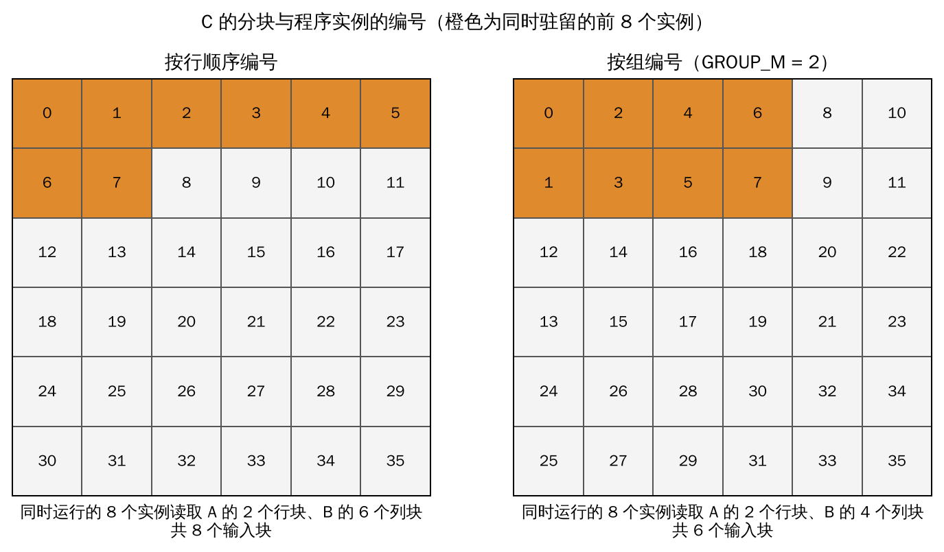
Figure 9.1　Two numbering schemes for $6 \times 6$ output blocks. Orange marks the first 8 concurrently running instances. Under row-major numbering they read 2 row blocks of $A$ and 6 column blocks of $B$; under grouping with $G = 2$ they read only 2 row blocks and 4 column blocks.

Take $g_m = g_n = 32$ and $W = 128$ as an example (roughly one instance per SM): row-major numbering needs $4 + 32 = 36$ input blocks, whereas with $G = 8$ only $8 + 16 = 24$ are needed, close to the lower bound $2\sqrt{128} \approx 22.6$. The Stax matmul template numbers with GROUP_M = 8, implemented by the first few lines of the template:

width = GROUP_M * grid_n
group_id = pid // width
group_size = min(grid_m - group_id * GROUP_M, GROUP_M)
pid_m = group_id * GROUP_M + (pid % group_size)
pid_n = (pid % width) // group_size

group_size handles the case where the last group has fewer than $G$ rows. This reordering changes the computation of no instance; it changes only their launch order, and therefore does not affect the result, only the cache behavior.

Tensor cores and mixed precision. The inner loop of the template is

acc = tl.dot(a, b, acc, allow_tf32=ALLOW_TF32, out_dtype=ACC_TYPE)

tl.dot is compiled by Triton into a matrix multiply-accumulate instruction on the tensor cores when the operands are float16, bfloat16 or float8; the accumulator type ACC_TYPE is always float32, which is consistent with the principle in Section 6.2that “half-precision operations are carried out in float32”. float32 operands go through the tensor cores only when ALLOW_TF32 is true: TF32 truncates the mantissa of an operand to 10 bits, so the relative error of a single rounding grows from $2^{-24}$ to about $2^{-11}$, while the accumulation still takes place in float32. Whether this is allowed is decided by the global matmul precision setting rather than by the template itself.

Tensor cores change where matrix multiplication sits on the roofline. On an H100 the nominal arithmetic throughput of the dense BF16 tensor cores is about 989 TFLOPS, so the ridge point is about $989 / 3.35 \approx 295$ FLOP/byte, which is 15 times the FP32 non-tensor-core ridge point (Figure 1.1, right). With $I_{\max} = 2n/(3b)$, a square matrix multiplication with $b = 2$ must have at least $n \ge 3 \times 295 \approx 885$ to become compute-bound; a smaller matrix multiplication is still limited by bandwidth even when it does use the tensor cores. This is also why epilogue fusion is more valuable in the era of tensor cores: the faster the matrix multiplication itself becomes, the larger the share of memory traffic taken by the pointwise operations that follow it.

Software pipelining. Each step of the inner loop has to read a pair of sub-blocks of $A$ and $B$ from main memory into the on-chip storage and then hand them to tl.dot. If reads and computation are serialized, every step waits for a full memory latency. With a pipeline depth num_stages of $s$, the on-chip storage provides $s$ sets of buffers for each operand, so that while step $t$ computes, the reads for steps $t+1$ through $t+s-1$ are already in flight. By Little’s law in Section 9.1, the bytes in flight must reach $\lambda B$ for the bandwidth to saturate, and increasing $s$ is precisely increasing the amount of traffic in flight per instance. The constraint comes from the on-chip storage capacity: each stage occupies $(B_M + B_N) B_K b$ bytes. Taking $B_M = B_N = 128$, $B_K = 64$ and BF16, each stage occupies 32 KB; with about 228 KB of configurable shared memory per SM on an H100, after deducting what the epilogue needs, $s$ is at most about 6. Together with the block sizes and the number of warps, $s$ enters the configuration space of Section 9.6and is chosen by measurement.

Hopper and later devices have a tensor memory accelerator (TMA), which moves an entire sub-block with a single instruction and notifies the computing threads when it completes. Stax provides a persistent TMA template for this purpose (triton_persistent_tma_mm): the grid size is taken as the number of SMs, and each instance loops over several output blocks, so that the epilogue of one block overlaps with the reads of the next.

9.9 CUDA Graphs

Every kernel launch has a fixed overhead $t_{\mathrm{launch}}$ paid by the host, of the order of microseconds. Issuing a launch on the host and executing the kernel on the device are asynchronous; suppose a region consists of $n$ kernels and the device execution time of the $k$-th is $t_k$, then the execution time of the region is about

When the kernels are short and $n \cdot t_{\mathrm{launch}} > \sum t_k$, the device idles between two launches and the execution time is decided by the host. Fusion reduces $n$, but it cannot remove this term. CUDA Graphs records a sequence of kernel launches as a single graph, which thereafter is submitted as a whole with one call, and the execution time becomes $T_{\mathrm{graph}} \approx t_{\mathrm{graph}} + \sum t_k$, where $t_{\mathrm{graph}}$ is essentially independent of $n$.

What is recorded is a definite sequence of launches: the kernel, the grid and the actual arguments (including the device pointers) of each launch are all fixed. Replaying is equivalent to re-executing the original program, and requires the following conditions:

1. The sequence of kernels, the grids and the shapes that the original program executes on the new input are the same as at recording time, that is, the control flow and the shapes do not depend on the data. Operators whose output shape depends on the data (such as nonzero, unique and masked_select), as well as operators that read a value on the device back to the host (such as item and tolist), violate this condition;
2. The new input resides at the addresses it had at recording time, or is copied to those addresses before the replay;
3. All computation within the region is on the same GPU, contains no host-side computation, and does not cross devices.

These three conditions have the same structure as the specialization of 第 Section 2: recording is a specialization of the “sequence of kernels and addresses”, and conditions 1 and 2 are its guards. Stax statically checks conditions 1 and 3 before wrapping and requires that the non-dynamic-shape mode be in effect; when they are not satisfied, it gives up on wrapping and the artifact executes as usual. Condition 2 is checked on every call: if the number of actual arguments, the shapes and the data pointers all match those at recording time, the graph is replayed, and otherwise this call directly executes the compiled artifact. If recording or replaying fails, the wrapper object enters a fallback state and thereafter always directly executes the compiled artifact.

The outputs of a replay lie in a memory pool dedicated to the graph, and the next replay writes to the same addresses, so results that the caller needs to keep across calls must be copied explicitly.

9.10 Attention

Attention is the most important family of operator combinations in modern models. Let the query, key and value of a single head be $Q \in \mathbb R^{N\times d}$, $K, V \in \mathbb R^{N\times d}$,

When it is executed operator by operator as defined, both $S$ and $P$ are matrices of $N \times N$ that must be written back to main memory and read out again. When the sequence length $N$ is much larger than the head dimension $d$ (the common values of $d$ are 64 or 128, and $N$ ranges from several thousand to several hundred thousand), the memory traffic of these two intermediate matrices far exceeds that of the inputs and outputs themselves.

Theorem 9.2 (The I/O Complexity of Attention [33])　Suppose the on-chip storage can hold $M$ elements, with $d \le M \le Nd$. Computing attention operator by operator requires $\Theta(Nd + N^2)$ main-memory accesses; a tiled single-pass algorithm requires $\Theta(N^2 d^2 / M)$. Moreover, for every $M$ in $[d, Nd]$, no algorithm that computes attention exactly can, in the asymptotic sense, do better than $\Theta(N^2 d^2/M)$.

Proof sketch　Operator by operator, $S$ and $P$ are each written out and read in once, contributing $\Theta(N^2)$. The tiled algorithm splits $Q$ by rows into blocks of size $B_r = \Theta(M/d)$, each of which stays resident on chip, and then scans $K$ and $V$ block by block along their row direction; each $Q$ block has to read all of $K$ and $V$, that is $\Theta(Nd)$, and there are $N/B_r = \Theta(Nd/M)$ such $Q$ blocks, for a total of $\Theta(N^2 d^2/M)$. Compared with the $\Theta(N^2)$ of the operator-by-operator implementation, the ratio is $d^2/M$: when the on-chip capacity $M$ is much larger than $d^2$, the tiled algorithm performs $M/d^2$ times fewer accesses. For example, with $d = 64$ and $M \approx 10^5$ it is about 24 times fewer; with $d = 128$ we have $d^2 = 16384$, and the same $M$ gives only about 6 times fewer, which is also why the larger the head dimension, the smaller the benefit of tiling. The proof of the lower bound can be found in [33]. $\square$

The tiled algorithm works precisely because of the online softmax of Section 9.5. For a query row $q$ and a segment of keys and values ${(k_j, v_j)}$, maintain the triple

The merge of two segments is

and after the scan has finished, $o = \mathbf a / \ell$. By the same argument as in Proposition 9.1, this operation is associative and commutative; the difference is that the second and third components are both rescaled by the same factor $e^{m_i - \mu}$. (Here $\mu$ denotes the maximum, to avoid confusion with the on-chip capacity $M$.) Attention can therefore be blocked, accumulated and split along the key direction exactly like a reduction: $S$ and $P$ appear on chip only as $B_r \times B_c$ blocks and are never written back to main memory (Figure 9.2).

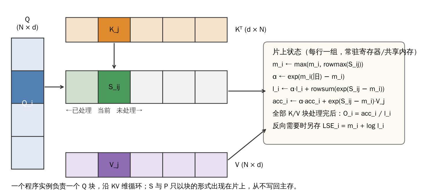
Figure 9.2　A single program instance of tiled attention. The instance is responsible for one $Q$ block, computes $S_{ij}$ block by block along the key-value direction, and updates the on-chip state $(m_i, \ell_i, \mathrm{acc}_i)$ with online softmax.

Backward pass and rematerialization. The backward pass needs $P$. Saving $P$ costs $\Theta(N^2)$ of storage, which is exactly what the tiled algorithm wants to avoid. The approach is the same as in 第 Section 5: instead of saving $P$, save only the per-row $\mathrm{LSE}i = m_i + \log \ell_i$ ($\Theta(N)$ numbers), and recompute $P{ij} = \exp(S_{ij} - \mathrm{LSE}_i)$ from $Q$, $K$ and the LSE during the backward pass. This is an extreme instance of “trading computation for storage” from Section 5.4: the price of the recomputation is one extra $QK^{\mathsf T}$, and what it buys is storage that drops from quadratic to linear. The difference lies in where the decision is made: it is written into the attention template rather than made automatically by the minimum cut on the joint graph, because the minimum cut can only choose which of the existing nodes to save and cannot invent a new intermediate quantity such as “save the LSE instead of $P$”.

Attention in Stax. Attention enters Stax along two paths.

The first is pattern matching. A handwritten expression such as softmax(q @ k.transpose(-2, -1) / s) @ v is recognized on the operator-level graph, rewritten into a scaled_dot_product_attention operator, and then handed to a dedicated implementation. Stax maintains 30 such patterns (graph_passes/fuse_attention.py), covering variants such as the scale written as a multiplication or a division, with or without dropout, with an additive mask, with the key transposed before or after, some of which are enabled only during inference. The limitation of pattern matching is just as obvious: as soon as the user’s code differs even slightly, for example by adding a positional bias before the softmax, the pattern no longer matches, execution falls back to the operator-by-operator fusion, and $S$ and $P$ still have to be written back to main memory.

The second is omni_attention, which turns “a variant of attention” itself into a programmable interface. The user describes a variant with two functions: score_mod(score, b, h, q_idx, kv_idx) modifies each score, and mask_mod(b, h, q_idx, kv_idx) decides whether a position takes part.

Listing 9.7　Causal attention with an ALiBi bias expressed with omni_attention

from tensorplay.nn.attention.omni_attention import omni_attention, create_block_mask

def causal(b, h, q_idx, kv_idx):
    return q_idx >= kv_idx

def alibi(score, b, h, q_idx, kv_idx):
    slope = tp.exp2(-(h + 1).to(tp.float32))       # 每个头一个斜率
    return score - slope * (q_idx - kv_idx)

block_mask = create_block_mask(causal, B=None, H=None, Q_LEN=4096, KV_LEN=4096, device="cuda")
out = tp.compile(omni_attention)(q, k, v, score_mod=alibi, block_mask=block_mask)

At compile time, score_mod and mask_mod are each traced into a small graph, lowered to a loop-level computation function, and embedded as a subgraph in the attention template: after a score block $S_{ij}$ has been computed and before the online softmax, the template calls this computation function for every element in the block. This is the same mechanism as the epilogue fusion of matrix multiplication in Section 9.8; the fusion point is simply in the middle of the template rather than at its end. The backward template embeds these two functions as well and automatically differentiates score_mod.

If mask_mod were evaluated elementwise, the masked-off positions would still have their scores computed and then discarded, saving no computation at all. create_block_mask therefore preprocesses the mask before the attention call: it evaluates mask_mod once at all $N^2$ positions to obtain a dense Boolean mask, and then reduces it per block (by default $128 \times 128$), dividing each block into three categories: fully visible full blocks, partially visible partial blocks, and entirely masked empty blocks, and records in a BCSR-like format the indices of the KV blocks that each $Q$ block needs to visit (kv_num_blocks, kv_indices, with the full blocks recorded separately in full_kv_num_blocks and full_kv_indices). The template traverses only the non-empty blocks, and calls mask_mod only on the partial blocks (Figure 9.3).

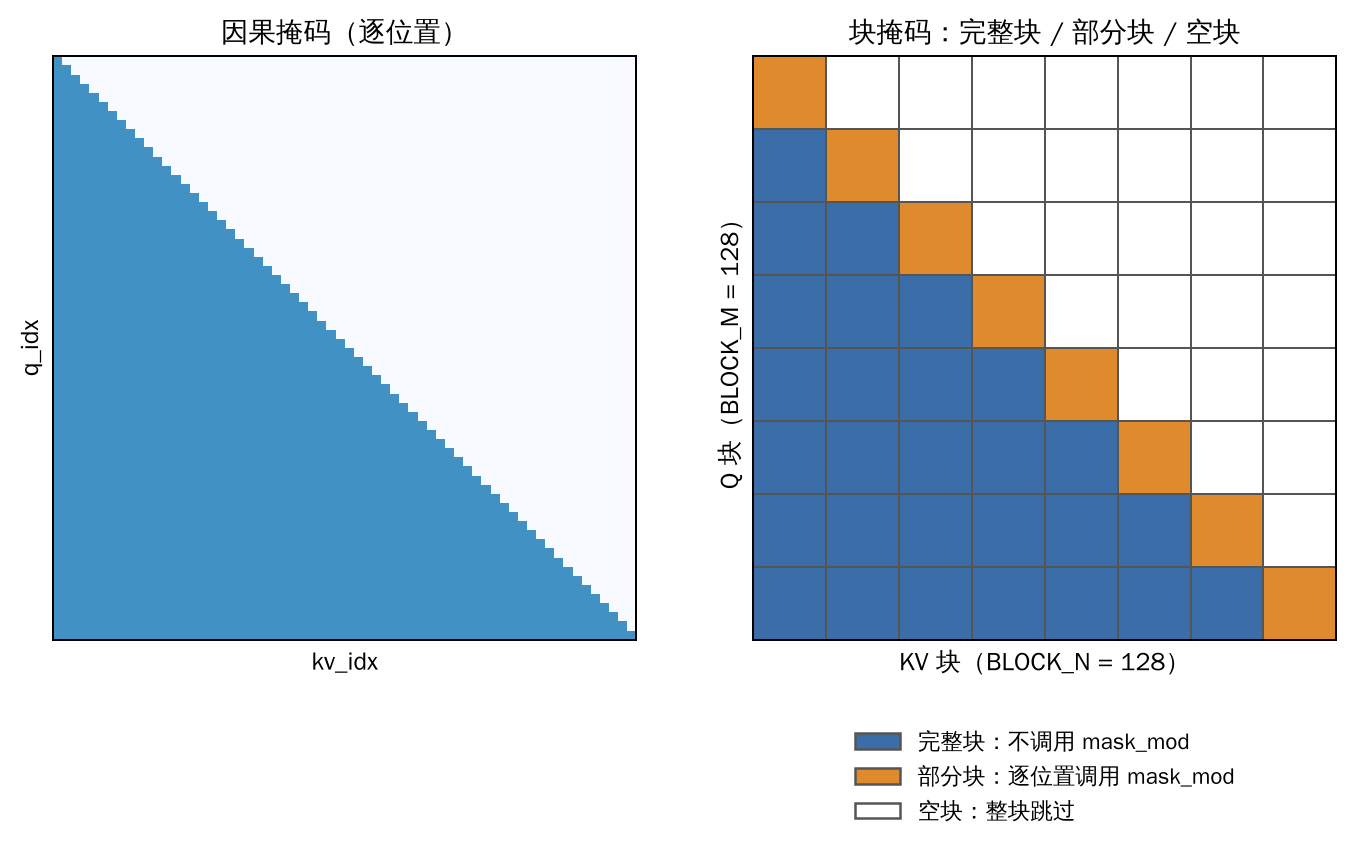
Figure 9.3　The block structure of a causal mask. Left: the per-position mask. Right: among the $8 \times 8$ blocks, the 8 on the diagonal are partial blocks, the 28 in the lower triangle are full blocks, and the 28 in the upper triangle are empty blocks.

For a causal mask, suppose there are $n$ blocks on each side; the blocks that need computing occupy $(n+1)/(2n)$, about half; and only the $n$ blocks on the diagonal need mask_mod to be evaluated, which is $1/n$ of all blocks. Constructing the block mask costs one $O(N^2)$ evaluation, but the constructed result has size only $O(n^2)$; it is independent of the concrete $Q$, $K$ and $V$, the same mask can be reused across layers and steps, and the construction cost is therefore amortized.

The attention template has several implementations, chosen according to the device and the shape: a general Triton template (omni_attention.py.jinja); a decoding template that splits along the KV direction to increase parallelism in decoding scenarios with very short queries (the basis for the split is still the associativity of online softmax, the same as the reduction splitting of Section 6.5); a FlashAttention template based on the CuTe DSL (experimental); and a C++ template for the CPU. The user can specify one of them with kernel_options={"BACKEND": ...}; if the specified implementation is unavailable, an error is raised rather than a silent fallback, which is consistent with the orientation of strict mode in Section 11.3.

10 Dynamic Shapes

All the previous sections have treated the shape as part of the specialization key (see Section 2.2): inputs of different shapes get different specialized versions, and within each version the shape is constant. This lets lowering and code generation substitute the shape into indices, loop ranges and all manner of heuristic criteria. The price is that a program whose shape changes often — for example, one whose batch size or sequence length varies with the input — has to be recompiled every time it meets a new shape. This section discusses how to let a single compiled artifact cover a class of shapes, and what this demands of each layer of the compiler stack.

10.1 Abstraction Levels of Shapes

Definition 10.1 (Shape Abstraction)　A shape abstraction is an equivalence relation on the shape space, and the shape component of the specialization key takes the equivalence class to which the input shape belongs. In order from fine to coarse, the three common shape abstractions are:

1. Concrete shape: two shapes are equivalent if and only if they are equal;
2. Symbolic shape: certain dimensions are declared variable and the rest take concrete values; shapes whose variable dimensions satisfy the same set of constraints within the declared ranges are equivalent to one another;
3. Rank: two shapes are equivalent if and only if they have the same number of dimensions.

The coarser the abstraction, the more inputs a single specialized version covers and the fewer compilations are needed; but the less shape information the compiler can exploit within each version. Coarsening is not always permitted, and Proposition 2.1 gives the constraint.

Proposition 10.1 (Reliability of Generalization)　Suppose the shape component takes the equivalence class of some shape abstraction. Reusing compiled artifacts under this key is reliable if and only if every compiled artifact is equivalent to the original function for every shape in its equivalence class.

Proof　The conclusion of Proposition 2.1 holds only for inputs with the same key. Inputs with the same key may have any shape in the equivalence class, so the artifact must be valid over the entire equivalence class; conversely, if the artifact is valid over the entire equivalence class, reuse yields the same result as recompilation. $\square$

Proposition 10.1 says that generalizing the specialization key is only half the problem; the other half is that the compiled artifact itself must be valid for a class of shapes, that is, that the generated code is shape-polymorphic. The former is a matter for the front end, whereas the latter concerns every layer of the compiler stack.

10.2 Symbolic Shapes and Shape Guards

A symbolic shape introduces a symbol $s$ for each variable dimension, carrying two pieces of additional information: the actual size of the example input at tracing time, called the hint value; and the declared range of values $[l, u]$. Arithmetic on shapes during tracing keeps its symbolic form; for example, flattening a tensor of $s \times 128$ gives a length of $128 s$. When the Python code needs to make a decision about a symbol, as in the branch if x.shape[0] > 32, the tracer evaluates the truth value from the hint value, continues along the corresponding branch, and records the decision made as a constraint. This is the same as the treatment of data-dependent control flow in Section 3.4; only the object of the decision changes, from the data of a tensor to its shape, and the constraint recorded is exactly the path condition in King’s sense [6].

Definition 10.2 (Shape Guard)　All the decisions made about symbols during tracing form a conjunction $\Gamma(s_1, \dots, s_k)$, called a shape guard. The compiled artifact is valid for every shape that satisfies $\Gamma$ and in which each symbol lies within its declared range.

After tracing ends, each guard has to be adjudicated against the declared range. The adjudication uses exactly the interval reasoning of Section 6.8, and there are three possible outcomes:

1. The range implies the guard; for example, if the declaration is $s \in [2, 4096]$ and the guard is $s \ge 1$, the guard is removed;
2. Some values in the range violate the guard, while the declarer requires the whole range to be valid; compilation fails with an error that gives a narrower range under which the declaration holds;
3. In all remaining cases the guard is kept as a runtime assertion of the compiled artifact.

Example 10.1　Export with tensorplay.export

def f(x, w):
    y = (F.relu(x + w) * 2).sum(-1)
    return y / x.shape[0]

Declare dimension 0 of x and w to be the same symbol $n \in [2, 4096]$. The exported graph is (counting annotations omitted):

add = x + w
relu = tensorplay_nn_functional_relu(add)
mul = relu * 2
sum_0 = mul.sum(-1)
getattr_0 = getattr_1(x, 'shape')
getitem = getattr_0[0]
truediv = sum_0 / getitem
_assert_dims_equal = tensorplay_export__trace__assert_dims_equal(w, 0, x, 0, 'n')
_assert_dim_range = tensorplay_export__trace__assert_dim_range(w, 0, 2, 4096, 'n')
return truediv

x.shape[0] is not replaced by the 64 of the example but is kept as a node in the graph, where it reads the actual size at every call. The end of the graph consists of two runtime assertions: dimension 0 of x and of w are equal, and lie within $[2, 4096]$. Calling it with an input whose dimension 0 is 10 gives a result of shape $(10,)$.

Example 10.2　If the function contains the branch if x.shape[0] > 32: and the declaration is $n \in [2, 4096]$, the 64 of the example makes the tracer take the true branch, and the guard is $n > 32$. This guard is violated by some of the values in the range, so exporting fails with an error:

Constraints violated (n)! The captured program holds only for some of the declared sizes:
  - Not all values of n in [2, 4096] satisfy the guard n > 32, which the program was captured under
Suggested fixes:
    n = Dim('n', min=33, max=4096)

After changing the declaration to $n \in [33, 4096]$ as suggested, the guard is implied by the range, the export succeeds, only the true branch is kept in the graph, and the range assertion at the end becomes $[33, 4096]$.

Symbolic shapes also bring a special difficulty: dimensions of size 1. The semantics of broadcasting depends on whether a dimension equals 1. Suppose dimension 0 of $x$ and of $y$ are the symbols $p$ and $q$ respectively. The result shape of x + y is: $p$ when $p = q$; $q$ when $p = 1$; $p$ when $q = 1$; and an error otherwise. Without any restriction, every binary operation would have to do a case analysis on the symbols.

Proposition 10.2　If the values of all variable dimensions are at least 2, then $p$ and $q$ can be broadcast if and only if $p = q$, and the resulting size is $p$.

Proof　When $p, q \ge 2$, neither of the cases $p = 1$ and $q = 1$ arises, leaving only the possibility $p = q$. $\square$

When making such decisions, TensorPlay’s export assumes that every variable dimension is at least 2, and therefore obtains $p = q$ by Proposition 10.2 and records it as a guard. Since this assumption is not itself declared, the guard is kept as a runtime assertion under outcome 3 above.

Example 10.3　Export b(x, y) = x + y, with dimension 0 of each of the two inputs declared variable. The resulting graph is:

add = x + y
getattr_0 = getattr_1(x, 'shape')
getitem = getattr_0[0]
getattr_2 = getattr_1(y, 'shape')
getitem_0 = getattr_2[0]
eq = getitem == getitem_0
_assert_shape_guard = tensorplay_export__trace__assert_shape_guard(eq, True, 'x.size()[0] == y.size()[0]')
return add

The guard $p = q$ introduced by the broadcasting rule becomes a runtime assertion. An alternative treatment is to specialize the two sizes 0 and 1 as concrete values in all cases and to use symbols only for sizes of 2 and above; PyTorch 2 takes this approach [15]. The two differ for an input of size 1: the former fails at the runtime assertion, whereas the latter compiles another version for it. TensorPlay’s export takes the former, while the dynamic mode of compile takes the latter (Section 10.4).

10.3 Backend Symbolization

After the front end has obtained a graph with symbolic shapes, the backends must generate code that is valid over the whole range. This affects almost every decision in 第 Section 6 to 第 Section 9.

First, index expressions become polynomials in the symbols. A contiguous tensor of shape $(s, 128)$ with strides $(128, 1)$ has the index $128 i_0 + i_1$; for shape $(128, s)$ with strides $(s, 1)$ the index is $s, i_0 + i_1$, where the coefficient is itself a symbol. The merging condition $a_j = s_{j+1} a_{j+1}$ of Proposition 6.3 must then be decided in the symbolic sense.

Second, loop ranges become runtime parameters. The element counts of a kernel can no longer be written as constants and must be passed in as parameters; and since whether $s$ is a multiple of the block size is unknown, the boundary masks cannot be omitted.

Third, size-dependent decisions must hold over the whole range. Such decisions are three-valued: true for every value in the range, false for every value, or undetermined. Suppose the value of an index expression when all loop variables take their maximum values is a polynomial $e(s_1, \dots, s_k)$ with nonnegative coefficients in the symbols. It is non-decreasing in each symbol, so

The criterion for 32-bit indices $\max e < 2^{31}$ therefore requires only substituting the upper bound of each symbol. If some symbol has no upper bound, the criterion cannot be determined, and one must either use 64-bit indices or add a guard $e < 2^{31}$ that excludes the offending shapes from this version. Persistent reduction (Section 9.4) requires the reduction length not to exceed an upper bound and must likewise be decided against the upper bound of the range; the number of segments in reduction splitting (Algorithm 6.1) and the threshold for materialization depend on the concrete size, so they can only be chosen by the hint value, and the chosen scheme is correct for every shape in the range but need not be optimal for all of them.

Fourth, the launch configuration is measured at the hint value. The measurements of Algorithm 9.1 are carried out on the shape corresponding to the hint value; the selected configuration is equally correct for other shapes, but its performance is not guaranteed. CUDA Graphs requires a fixed shape (condition 1 in Section 9.9), which is incompatible with symbolic shapes.

It follows that symbolic shapes put correctness first: any size-dependent optimization must either hold over the whole range, be restricted by a guard, or fall back to a conservative choice. Shape-polymorphic artifacts buy fewer compilations at the price of constant indices, unmasked loops and configurations tailored to particular shapes.

10.4 How TensorPlay Handles This

By default, TensorPlay’s compile uses concrete shapes. The argument dynamic=True coarsens the shape component of the specialization key to rank. By Proposition 10.1, whether this coarsening is reliable depends on whether the backend can generate shape-polymorphic artifacts, so TensorPlay distinguishes two cases according to whether the backend declares support for symbolic capture (supports_symbolic_shapes).

For a backend that does not support symbolic capture, such as the debugging backend in Section 11.4, the region is still traced by run-time sampling as in Section 3.3, with one correction added: if the function reads the shape, len or ndim of some input, the complete shape of that input re-enters the specialization key, because the size read during tracing has already been written into the graph as a constant. Such a backend executes operator by operator, so the artifact is itself shape-polymorphic.

Stax declares support for symbolic capture, and under dynamic=True the handling is divided into four steps: capture, lowering, guards and caching.

Capture. The region is captured by the symbolic shape tracer: one symbol is introduced for every dimension of every input tensor, with the hint value taken from the size in the example. Dimensions of size 0 or 1 introduce no symbol and are specialized as concrete values, which is the second approach described at the end of Section 10.2. Reading shape, size() and numel() yields symbolic expressions, and shape arithmetic stays in symbolic form; for example, the dimension inferred in x.reshape(x.size(0), -1) is a run-time integer division. Decisions about shapes are evaluated with the hint value, continue along the corresponding branch, and are recorded as the guards of Definition 10.2. Reading a shape therefore no longer lets the complete shape enter the specialization key; only tensor inputs nested inside containers such as tuples and lists, as well as external calls whose output metadata has concrete values, are still specialized with concrete shapes.

Lowering. Lowering takes place in a shape environment, in which indices, loop ranges and strides are the symbolic expressions described in Section 10.3. The CPU kernels (C++) and the GPU kernels (Triton) share one set of lowering rules and one shape environment, so both acquire shape polymorphism at the same time: on every call the generated kernels bind their sizes and strides from the actual arguments. Slicing preserves symbolic lengths, strides and offsets, including positive strides, negative bounds and bounds computed from the input size; integer indexing and select use guards to ensure that the index lies in range; and the returned views share storage with the inputs.

Guards. Every artifact carries a guard function, which is the conjunction of two parts:

1. Capture guards: the decisions made about shapes during tracing (the $\Gamma$ of Definition 10.2), together with the dimensions specialized as concrete values (those of size 0 or 1);
2. Input guards: the layout assumptions made during lowering, including the rank and the storage offset of each input, that the size and stride of each dimension equal the corresponding symbolic expressions, that every symbolic dimension is at least 2, and the guards and runtime assertions recorded by the shape environment during lowering.

Both parts are generated at compile time as a Python function that reads only metadata and holds no example tensor. During forward capture, dimensions whose hint values are equal share one symbol, and this equality is itself part of the input guards, so it is never assumed without being checked.

Caching. In dynamic mode the specialization key contains no sizes, so multiple artifacts can hang under the same key, each corresponding to a different set of guards. At call time the artifacts for the key are taken and their guards checked; when they do not hold, the other artifacts under the same key are searched for one whose guards do hold; and only when none holds is a recompilation performed. All artifacts count towards the limit on the number of specializations; once that limit is reached, unless fullgraph is set (in which case an error is raised), a newly compiled artifact executes as usual but is no longer stored in the cache, and every cache miss triggers a fresh compilation, up to the limit on the cumulative number of compilations (Section 2.4).

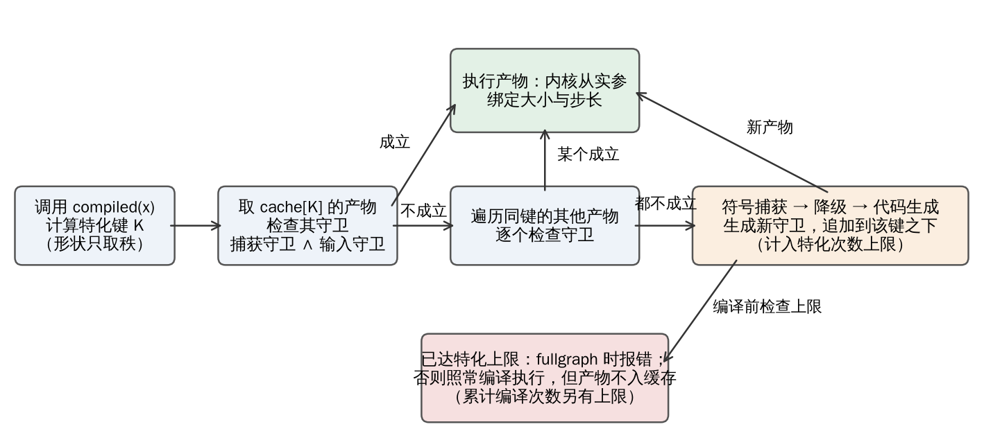
Figure 10.1　The dispatch of one call in dynamic mode. Multiple artifacts can exist under the same specialization key, each with its own set of guards.

Example 10.4　For

def fn(x):
    return x + 1 if x.shape[0] > 4 else x * 2

compiled = tp.compile(fn, dynamic=True, strict_native=True)
for n in (3, 7, 2, 9, 4, 11):
    compiled(tp.arange(n, dtype=tp.float32))

The six calls generate only two artifacts. Capture happens at $n = 3$, with the guard $n \le 4$; at $n = 7$ that guard does not hold, so capture happens again, giving a version with the guard $n > 4$; from then on every call hits one of these two. Similarly, calling lambda x: x * 2 + 1 with the sizes 3, 1, 0, 7, 1, 0 and 11 in that order generates three artifacts, corresponding to $n \ge 2$, $n = 1$ and $n = 0$ respectively; calling alternately on a contiguous tensor and on its transpose, whose stride relations differ, generates two artifacts.

Training. A training region goes through the joint graph and the partitioning of Section 5, and the forward and backward passes each lower to one shape-polymorphic artifact, with compatible sizes sharing this pair of artifacts. The dimensions needed by the backward pass are not written as constants but are saved by the forward pass as symbolic scalar values; every forward call saves its own dimensions for the backward call that corresponds to it later. The input dimensions of the backward graph are mutually independent, and are not merged into one symbol even when their values on the example happen to be equal. The gradient formulas (config/derivatives.yaml and the native TPX nodes) are correspondingly changed to compute in terms of the symbolic sizes, covering pointwise operations, the sum and mean reductions, broadcasting, reshape and expand, squeeze, slicing and select, unflatten, diagonal and repeat; the gradients of variance and standard deviation, including the case where the mean is also output, compute the reduction counts from the run-time dimensions. When an artifact falls back to interpreted execution, the native TPX gradients likewise compute from the run-time dimensions.

There remain three kinds of case that still fall back to specialization by size: a gradient formula saves concrete shape metadata, scalar operands or operator parameters derived from shapes, as in (x / x.shape[0]).sum(), and another version with a guard is chosen when these values change; when the correction term of the variance is greater than 1, specialization is used in order to preserve the test for non-positive degrees of freedom; and when the broadcasting pattern or the stride layout differs, as in Example 10.4, another artifact is chosen.

Fallback and limitations. Without strict_native=True, a region whose code cannot be generated executes its graph interpretively, and the capture guards are checked as usual; with it, an error is raised instead (Section 11.3). CUDA Graphs requires a fixed shape and is therefore not used for wrapping in dynamic mode (Section 9.9). Symbolic capture can also be used on its own through make_graph(..., tracing_mode="symbolic"), but this entry point does not yet support the tracing of storage-free pseudo-tensors, nor operators whose output size depends on the data. The export of Section 10.2remains another path: it adjudicates the guards against the declared range and leaves the size-1 case to a runtime assertion.

In concrete-shape mode, and for the dimensions that must still be specialized as described above, the usual way of bounding the number of compilations is bucketing: rounding the variable dimensions up to a few pre-selected sizes.

Proposition 10.3　Suppose the values of the variable dimensions lie in $[m, M]$, with $m \ge 1$, and the buckets are powers of two, so that a size $n$ is rounded up to $2^{\lceil \log_2 n \rceil}$. Then there are at most $\lceil \log_2 M \rceil - \lfloor \log_2 m \rfloor + 1$ specialized versions, and the rounded-up size is less than $2n$.

Proof　The rounded-up sizes range over ${2^j : \lfloor \log_2 m \rfloor \le j \le \lceil \log_2 M \rceil}$, whose cardinality is as stated. And $2^{\lceil \log_2 n \rceil} < 2^{\log_2 n + 1} = 2n$. $\square$

The padded elements must be handled with masks or with the identity element so that they do not affect the result, for example by filling with the identity element in a reduction and by masking them off in attention. Proposition 10.3 gives one kind of trade-off between the number of compilations and the redundant computation: the smaller the common ratio of the buckets, the less redundancy and the more versions.

10.5 Data-Dependent Shapes

All the symbols discussed so far come from the shapes of the inputs, and a hint value from the example is available at tracing time. There is another class of operators whose output shape depends on the data of the input: the number of rows of the output of nonzero is the number of nonzero elements, the length of the output of unique is the number of distinct values, and the length of masked_select is the number of true entries in the mask. Such sizes can be computed from the example at tracing time, but the value on the example is in no way representative: the number of nonzero entries of the next call has nothing to do with that of this one.

The standard way of handling such sizes is to introduce a symbol $u$ without a hint (PyTorch 2 calls this an unbacked symbol): it carries only the known constraints, such as $0 \le u \le N$, and no example value. Any decision about $u$ cannot be evaluated on the example and can have only two outcomes: it follows from the known constraints (for instance, u >= 0 is always true when $u \ge 0$), or it cannot be determined. An undetermined decision cannot become a guard, because a guard is a path condition recorded by evaluating on the example, and $u$ has no example; it can only raise an error, or require the user to state the constraint explicitly with an assertion such as tensorplay._assert, turning the decision into a run-time check.

Proposition 10.4　Suppose the symbol $u$ carries only a constraint set $\mathcal C$. If the compiler makes the decision $\varphi$ only when $\mathcal C \models \varphi$ or $\mathcal C \models \neg\varphi$, and otherwise refuses to compile, then for every $u$ satisfying $\mathcal C$ the execution path of the compiled artifact is the same as that of the original program.

Proof　Every decision made by the compiler takes the same truth value for all $u$ satisfying $\mathcal C$, so the path the artifact follows is, for these $u$, the path the original program would actually take. By the argument of Proposition 2.1, the artifact is equivalent to the original program. $\square$

The condition of Proposition 10.4 is far stricter than a shape guard: a shape guard allows “make the decision on the example and check afterwards”, whereas a symbol without a hint allows only “decisions that can be proved in advance”. This leaves data-dependent shapes severely constrained in the backends. For example, for the pointwise operations after x[nonzero(x)], the loop range is $u$ and a masked loop can be generated as usual; but if the subsequent code compares $u$ with some constant in order to choose a reduction strategy, the comparison cannot be determined and the compiler must pick the conservative scheme that is correct for every $u$.

TensorPlay’s current handling is simpler. The lowering of Stax registers operators such as nonzero, unique and bincount as fallback kernels (Section 6.1), which the framework executes as they are, with their output shapes determined at run time; the part after a fallback kernel can still be compiled, but the shapes in it that depend on that size can only be specialized as concrete values. The symbolic capture entry point of Section 10.4does not support operators whose output size depends on the data (make_graph(..., tracing_mode="symbolic") raises an error on them). For such operators, the CUDA Graphs of Section 9.9do not apply either, because the output size cannot be fixed at recording time.

Previous: Part Three　Scheduling, Fusion and CPU Code Generation　｜　Table of Contents　｜　Next: Part Five　Caching, Discussion, Models and Measurements; Summary and Exercises