Previous: Part Two Automatic Differentiation and Lowering | Table of Contents | Next: Part Four GPU Code Generation and Dynamic Shapes
Reference numbers [n] used in this chapter are listed in Part Six; section numbers, theorem numbers, and exercise numbers are numbered uniformly across the whole chapter, so cross-section references remain valid as usual.
7 Scheduling and Fusion
After lowering is complete, every buffer written to memory is a potential kernel. The scheduler decides in what order these buffers are computed, which of them are merged into the same kernel, and supplies dependence and lifetime information to code generation. The function composition of Section 6.3has already fused pointwise operations with one another; the fusion discussed in this section occurs between materialized buffers, for example a reduction and the broadcast that follows it, or several reductions reading the same input.
7.1 Dependences
The scheduler creates one scheduling node per buffer. A handler that records reads and writes executes its computation function (Section 6.7), yielding the positions it reads and writes.
Definition 7.1 (Dependence) The dependence of node $b$ on node $a$ is written $a \to b$, meaning that $b$ must execute after $a$. There are three kinds of dependence. A memory dependence records the buffers accessed, the index expressions of the accesses, and the range of each loop variable. A whole dependence records only the buffer and is used for external calls whose indices cannot be analyzed. A weak dependence carries no data and constrains only the ordering; it is used to ensure that the node reading a buffer is scheduled before the node rewriting it in place.
The indices in a memory dependence are what fusion decisions are based on: if $b$ reads a position written by $a$, and their index expressions coincide under the same loop variables, then the data each iteration of $b$ needs is produced by exactly the corresponding iteration of $a$, so the two can be merged into one loop and the intermediate value need never leave registers or cache. Each node also records its iteration grouping, that is, the pair (pointwise range, reduction range).
The iteration grouping determines whether two nodes can share one loop nest.
Definition 7.2 (Compatibility of Iteration Spaces) Let the iteration grouping of a node be $(n, r)$, where $n$ is the number of elements in the pointwise iteration and $r$ is the number of elements reduced for each output; a pointwise node has $r = 1$. Two nodes’ iteration spaces are called compatible if one of the following conditions holds:
- Both are reductions, and $n_1 = n_2$ and $r_1 = r_2$;
- Both are pointwise nodes, and $n_1 = n_2$;
- One is a pointwise node $(N, 1)$ and the other a reduction $(n, r)$, and either $N = n$, or $N = n r$ and the pointwise node’s iteration range can be split into two groups of $n \times r$.
The two cases of condition 3 correspond to the two kinds of pointwise operation, before and after a reduction. When $N = n$, the pointwise operation is performed once per output, for example taking the reciprocal of the row sums; when $N = nr$, the pointwise operation traverses as many elements as the reduction, for example dividing every element of each row by the row sum in Example 7.1. The latter requires that the pointwise node’s iteration range be splittable according to the shape of the reduction: the $64 \times 128$ pointwise node of Example 7.1 happens to split into 64 outputs of 128 elements each. The GPU backend decides compatibility by element count; the CPU backend keeps the full per-dimension ranges and decides by whether the outer loops agree (Example 7.1, Example 7.2).
In-place modification is handled by renaming: if some kernel overwrites buffer buf0 and produces buf1, then every subsequent use of buf0 is treated as a use of buf1. This works the same way as in the construction of SSA and keeps the dependence graph acyclic.
Example 7.1 Let k(x) = x / x.sum(-1, keepdim=True), with $x$ of shape $64\times128$. After lowering there are two nodes, and the dependences before fusion are as follows (CPU; the prefix and some fields are omitted):
op0: SchedulerNode(ComputedBuffer)                     # 按行求和
op0.writes = [MemoryDep('buf1', c0, {c0: 64})]
op0.met_dependencies = [MemoryDep('primals_1', c0, {c0: 8192})]
op0.group.iteration = ((64,), (128,))

op1: SchedulerNode(ComputedBuffer)                     # 逐元素相除
op1.writes = [MemoryDep('buf2', c0, {c0: 8192})]
op1.unmet_dependencies = [MemoryDep('buf1', c0, {c0: 64})]
op1.met_dependencies = [MemoryDep('primals_1', c0, {c0: 8192})]
op1.group.iteration = ((64, 128), ())
op0 is a reduction, with an iteration grouping of 64 outputs each reducing 128 elements; op1 is a pointwise operation, with an iteration grouping of $64\times128$ and no reduction. The dependence of op1 on buf1 is not yet satisfied, so it must be scheduled after op0. The indices in the dependences have already been normalized: the two-dimensional index 128*i0 + i1 of primals_1 is collapsed into the one-dimensional c0, whose range is 8192.
7.2 The Fusion Problem
Definition 7.3 (Fusion Scheme) Let the dependence graph be $D = (V, E)$. A partition $\mathcal P = {P_1, \dots, P_m}$ of $V$ is called a fusion scheme if:
- The nodes in each block $P_j$ have pairwise compatible iteration spaces (Definition 7.2) and can be generated as one and the same kernel;
- The quotient graph $D / \mathcal P$ obtained by contracting each block into a single vertex is acyclic.
The cost of a fusion scheme is the sum of the transfer volumes between the kernels and main memory.
Condition 2 guarantees that a legal execution order exists for the kernels: if the quotient graph had a cycle, two kernels would be predecessors of each other, and whichever ran first would find some data not yet produced. Minimizing the cost is NP-hard for fusion schemes in general [20, 55]. Below is a complete proof under the cost model of Definition 7.3. Abstracting away the details of the iteration spaces, record as forbidden node pairs those pairs that cannot go into the same block; they arise from incompatibility of iteration spaces (Definition 7.2) or from an illegal dependence distance (Proposition 7.3 later in Section 7.2). A buffer that has a user outside the block of its producer must be written out once, and is read in once by each other block that contains one of its users.
Theorem 7.1 (NP-Hardness of Fusion) Given a directed acyclic graph, the size of each node’s output, and a set of forbidden node pairs, deciding whether there exists a fusion scheme of cost at most $K$ is NP-complete. The conclusion still holds even if every edge in the graph goes from a source to a sink and there are only three forbidden node pairs.
Proof It is in NP: given a partition, checking the forbidden pairs, the acyclicity of the quotient graph, and computing the cost are all polynomial.
NP-hardness: by reduction from the three-terminal multiway cut problem. That problem gives an undirected graph $H = (V, E)$ with nonnegative edge weights $w$ and three terminals $s_1, s_2, s_3$, and asks whether there is an edge set $E’$ of total weight at most $K’$ such that after deleting $E’$ the three terminals are pairwise disconnected; it is NP-complete [41]. Construct $D$ as follows: every vertex $v \in V$ corresponds to a sink $n_v$ with output size 0; every edge $e = {u, w}$ corresponds to a source $x_e$, which is a computation node (reading only one external input of size 0), has output size $w(e)$, and is read by $n_u$ and $n_w$; the forbidden pairs are ${n_{s_i}, n_{s_j}}$ for $i < j$. Set $K = 2K’$. It suffices to prove that the minimum fusion cost is exactly twice the weight of a minimum multiway cut.
($\ge$) Take any feasible fusion scheme. Group $V$ by the block containing $n_v$; the three terminals fall into different groups. Let $E’$ be the set of edges whose two endpoints lie in different groups. Every connected component of $H - E’$ lies within one group, so $E’$ is a multiway cut. For each $e \in E’$, the two users of $x_e$ lie in different blocks, so at least one of them is not in the block of $x_e$; the buffer of $x_e$ must be written out once and read in at least once, costing at least $2w(e)$. The cost of the scheme is therefore at least $2w(E’)$, and hence at least twice the weight of a minimum multiway cut.
($\le$) Take any multiway cut $E’$, number the connected components of $H - E’$ arbitrarily as $1, \dots, r$, and write $\mathrm{comp}(v)$ for the number of the component containing $v$. Let block $j$ be ${n_v : \mathrm{comp}(v) = j} \cup {x_e : e = {u, w},\ \min(\mathrm{comp}(u), \mathrm{comp}(w)) = j}$. The three terminals lie in different components, so the forbidden pairs are satisfied. Every cross-block edge goes from an $x_e$ to an endpoint $n$, and the number of the block containing the former is the smaller of the two endpoint numbers, so every cross-block edge goes from the lower-numbered block to the higher-numbered one and the quotient graph is acyclic. An $x_e$ whose two endpoints lie in the same component shares a block with its users, and the cost is 0; an edge whose two endpoints lie in different components must belong to $E’$, and the cost is $2w(e)$. The cost of the scheme is therefore at most $2w(E’)$. $\square$
Theorem 7.1 allows arbitrarily given forbidden pairs; the forbidden pairs in Stax are determined by iteration spaces and dependence distances and carry more structure, and the theorem does not answer whether this restricted problem class is still NP-hard (Exercise 45). In practice Stax uses a greedy algorithm that merges one pair of nodes at a time while maintaining condition 2.
When does merging a pair of nodes destroy acyclicity? The following proposition gives a test.
Proposition 7.1 Let $D$ be a directed acyclic graph and $a, b \in V$. After $a$ and $b$ are merged into a single vertex, the resulting graph contains a cycle if and only if there exists in $D$ a directed path from $a$ to $b$ (or from $b$ to $a$) that passes through a third vertex.
Proof If a path $a \to c \to \cdots \to b$ exists, then after the merge $c$ is both a successor and a predecessor of the new vertex, forming a cycle. Conversely, suppose the merged graph has a cycle. The cycle must pass through the new vertex (otherwise the cycle already existed in $D$), and the part of the cycle that leaves the new vertex and returns to it is a path in $D$ from ${a, b}$ to ${a, b}$; it cannot go from $a$ back to $a$ or from $b$ back to $b$ ($D$ is acyclic), and it cannot be the single edge $a \to b$ or $b \to a$ (such an edge becomes an intra-block edge after the merge and does not appear in the quotient graph), so it is a path through a third vertex connecting $a$ and $b$. $\square$
The condition of Proposition 7.1 can be reduced to a query on ancestor sets. Write $\mathrm{anc}(v)$ for the set of vertices that can reach $v$ in $D$. A path through a third vertex $c$ connecting $a$ and $b$ exists if and only if
$$\exists\, c \notin \{a, b\}:\quad c \in \mathrm{anc}(a) \cup \mathrm{anc}(b)\ \text{且}\ \{a, b\} \cap \mathrm{anc}(c) \ne \varnothing,$$that is, $c$ is an ancestor of one of them and a descendant of the other. Before fusion begins, the scheduler computes the ancestor set of every node once. During fusion, new ancestor relations can only arise through nodes that have already been fused, so a query only has to search upward along already-fused nodes, and the transitive closure of the whole graph need not be recomputed after every merge.
Vertical fusion must further guarantee that the merged execution order is still correct.
Proposition 7.2 (Correctness of Vertical Fusion) Let $a \to b$, where the index at which $a$ writes buffer $B$ is the injective $w(i)$, with $i$ an outer iteration variable of $a$. If every read of $B$ by $b$ has index exactly $w(i)$, where $i$ is a prefix of $b$’s iteration variables, then executing in the order “for each $i$, first execute the $i$-th iteration of $a$, then execute all iterations of $b$ whose prefix is $i$” gives the same result as first finishing $a$ and then running $b$.
Proof An iteration of $b$ whose prefix is $i$ reads only position $w(i)$. Since $w$ is injective, that position is written only by the $i$-th iteration of $a$; in the fused order, this write completes before those reads and is never overwritten afterwards. The value read by $b$ is therefore the same as in the original order. The writes of $b$ are not read by $a$ (otherwise both $a \to b$ and $b \to a$ would hold, contradicting acyclicity), so the result of $a$ is unchanged as well. $\square$
Example 7.1 is exactly this situation: $a$ is the row sum with $w(i) = i$; $b$ is the pointwise division, with iteration variables $(i, j)$ and an index for reading the row sums that is the prefix $i$. The “prefix” in the proposition lets $b$ have an inner dimension that $a$ does not, which corresponds to broadcasting the reduction result back over the entire row. If the index read is not equal to $w(i)$, for example if $b$ reads the $i+1$ output of $a$, then after fusion the read would happen before the write, and vertical fusion is rejected.
Proposition 7.2 handles only the case where the read index is exactly the write index. The general case needs the notion of a dependence distance, a basic tool of loop transformation theory [29].
Definition 7.4 (Dependence Distance) Suppose the $i$-th iteration of $a$ writes position $w(i)$ of buffer $B$, where $w$ is injective, and the $j$-th iteration of $b$ reads position $r(j)$. If $r(j)$ lies in the image of $w$, write $p(j) = w^{-1}(r(j))$ for the iteration of $a$ that produces that value. After aligning the iteration spaces of $a$ and $b$ on common outer dimensions, $\delta(j) = p(j) - j$ is called the dependence distance of the $j$-th iteration of $b$ on $a$, compared lexicographically.
Proposition 7.3 (Legality of Fusion) Let the iteration spaces of $a$ and $b$ be compatible and aligned on common outer dimensions, and after fusion execute the corresponding iterations of $a$ and $b$ in turn for each outer index.
- If the fused loop executes sequentially, fusion preserves semantics if and only if $\delta(j) \preceq 0$ for all $j$, that is, every value read is produced by an iteration no later than the reader;
- If the fused outer iterations execute in parallel with no ordering guaranteed among them, fusion preserves semantics if and only if $\delta(j) = 0$ for all $j$.
Proof (1) Under sequential execution, before the $j$-th iteration of $b$ executes, the $0, \dots, j$ iterations of $a$ have all completed. If $\delta(j) \preceq 0$, the iteration $p(j) \preceq j$ that produces $r(j)$ has already executed, so the value read by $b$ is the same as in the original order. Conversely, if some $\delta(j) \succ 0$, then $p(j)$ executes only after $j$, and $b$ reads the contents as they were before the write, which differs from the original program. (2) Under parallel execution the order among distinct outer iterations is arbitrary, and only the “first $a$, then $b$” order inside a single outer iteration is guaranteed. When $\delta(j) = 0$ the value is produced within the same iteration and the read is correct; when $\delta(j) \ne 0$ there is always a schedule in which $p(j)$ executes later than $j$, and the read is wrong. $\square$
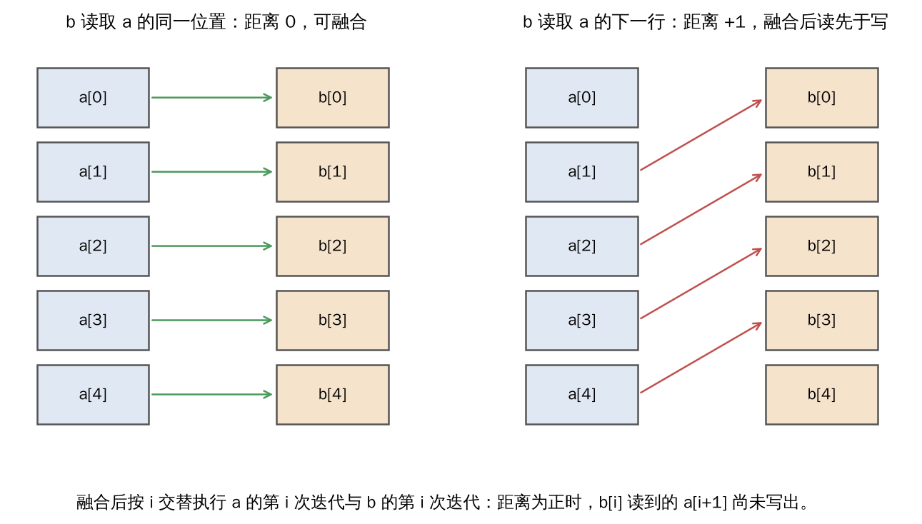
Figure 7.1 Dependence distance. Left: the distance is 0, and each $b[i]$ reads only the $a[i]$ written by the same iteration. Right: the distance is $+1$, and the $a[i+1]$ that $b[i]$ reads after fusion has not been written yet.
Proposition 7.2 is exactly the case $\delta \equiv 0$ of item 2 of Proposition 7.3. The kernels Stax generates are parallel in the outer dimensions (an OpenMP loop on the CPU, a program instance on the GPU), so it requires the read and write indices to be exactly equal after normalization, and dependences with negative distance, although legal under sequential execution, are rejected as well. Cases where the distance is negative and fusion is nonetheless required, such as reading adjacent positions in a template convolution, must introduce synchronization or overlapping tiles inside the kernel, which lies outside the model of the Stax scheduler.
Deciding the sign of $\delta$ requires solving $w(i) = r(j)$. When the indices are affine functions of the loop variables, this is a system of integer linear equations together with the inequality constraints given by the loop ranges. The classical dependence tests answer it at progressively greater cost: the GCD test only checks whether the equations have an integer solution; the Banerjee test checks the inequalities over a real relaxation; the Omega test [30] decides integer feasibility exactly by Fourier–Motzkin elimination, exponential in the worst case. The polyhedral model [31] pushes this approach to its extreme (its fundamental theorem is given in Section 7.7): iteration spaces and dependences are both represented as integer polyhedra, and the fusion, tiling, interchange, and skew of loops are expressed uniformly as affine schedules, with integer linear programming choosing among the legal schedules the one that optimizes an objective function; PLUTO [32] minimizes dependence distances as its objective and thereby obtains parallelism and locality at the same time.
Stax does not adopt the polyhedral model. Its dependence test only compares whether the normalized index expressions are symbolically equal (the simplification of Section 6.8brings different spellings to the same form), and unequal means not fusable. The test is conservative: it never accepts an illegal fusion, but it does reject a portion of the legal fusions, such as sequential fusion with negative distance and fusion that would be legal only after a loop skew. What is bought in return is analysis time linear in the size of the expressions, with no integer program to solve, which matters for a just-in-time compiler that has to process hundreds of nodes on every compilation.
7.3 The Greedy Fusion Algorithm
Algorithm 7.1 Greedy Fusion
输入:调度节点集合 V
输出:融合后的节点集合 V
1  for round = 1 to 10:
2      C ← 共享至少一个缓冲区的节点对
3      C ← {(a, b) ∈ C | can_fuse(a, b)}
4      将 C 按 score(a, b) 降序排列
5      for (a, b) in C:
6          若 a、b 本轮均未被合并,且由命题 7.1 合并不产生环:
7              V ← (V − {a, b}) ∪ {fuse(a, b)}
8      若 |V| 未减少,则终止
9  return V
Line 2 generates candidates only among nodes that share a buffer. Two nodes that share no data do not reduce memory accesses when fused, and excluding them makes the candidate set far smaller than $|V|^2$.
The legality test on line 3 distinguishes two kinds of fusion. If $b$ reads a buffer written by $a$, it is called vertical fusion, and after fusion the result of $a$ need not be written to main memory; if the two merely read the same input, it is called horizontal fusion, and after fusion the shared input only has to be read once. The conditions of the test include: compatible iteration spaces (Definition 7.2); for vertical fusion, read and write indices satisfying the condition of Proposition 7.2; at most 128 nodes after fusion and at most 32 distinct buffers involved; a number of shared data bytes no lower than a threshold; fusion does not extend excessively the lifetime of the input the two share, which would significantly raise peak memory; two reductions that require a strict reduction order cannot be fused; the two are not on different execution streams.
The core of the benefit function on line 4 is the number of bytes of shared data: the sum of the byte counts of the dependences that two nodes share with identical indices is exactly the main-memory traffic saved by the fusion. Benefits are compared lexicographically. Let the score of a candidate pair be $(\tau, \sigma, \omega, -\delta)$: $\tau$ is a type score, equal to 1 when the two are both reductions or both pointwise nodes and share data, and 0 otherwise; $\sigma$ is the number of main-memory bytes saved; $\omega$ is the number of shared buffers; $\delta$ is the distance between the two in the original order. There is one exception: when the $\sigma$ of two candidates differs by more than a factor of 16, only $\sigma$ is compared. The fusion of a template with its epilogue is ordered after ordinary fusion (Section 9.8). The type score comes before the byte count because nodes of the same type produce a simpler loop structure after fusion; the distance comes last because the farther apart the two are, the more the fusion extends the lifetime of the data or result read by the earlier node, increasing peak memory.
The greedy algorithm does not guarantee optimality: merging the highest-scoring pair first may make another combination illegal whose score is slightly lower but better in aggregate. The algorithm repeats in rounds; within a round a node takes part in at most one merge, and the number of rounds is capped at 10.
7.4 A Fusion Example
Example 7.1 (continued) For the two nodes of k, the fusion log reads, in its essential part:
found 1 possible fusions
fusing op0 with op1
op0_op1: OuterLoopFusedSchedulerNode(SchedulerNode,SchedulerNode)
The two share primals_1 and buf1, and the shared data scores 33024, exactly the 32768 bytes of primals_1 (8192 floats) plus the 256 bytes of buf1 (64 floats). Since the iteration grouping of op0 is ((64,), (128,)) and that of op1 is ((64, 128), ()), their outer 64 iterations coincide, so the CPU backend decides an outer-loop fusion depth of 1 and fuses them into a single outer-loop-fused node. The generated kernel is shown in Listing 7.1.
Listing 7.1 The fused kernel of Example 7.1 (CPU; namespaces and bounds checks omitted)
#pragma omp for
for (int64_t x0 = 0; x0 < 64; x0 += 1) {
    // op0:第 x0 行求和
    float tmp_acc0 = 0;
    Vectorized<float> tmp_acc0_vec = Vectorized<float>(0);
    for (int64_t x1 = 0; x1 < 128; x1 += 16) {
        auto tmp0 = Vectorized<float>::loadu(in_ptr0 + 128*x0 + x1, 16);
        tmp_acc0_vec = tmp_acc0_vec + tmp0;
    }
    tmp_acc0 = tmp_acc0 + vec_reduce_all<float, 1>(add, tmp_acc0_vec);
    out_ptr0[x0] = static_cast<float>(tmp_acc0);
    // op1:第 x0 行逐元素相除
    for (int64_t x1 = 0; x1 < 128; x1 += 16) {
        auto tmp0 = Vectorized<float>::loadu(in_ptr0 + 128*x0 + x1, 16);
        auto tmp1 = out_ptr0[x0];
        auto tmp2 = Vectorized<float>(tmp1);
        auto tmp3 = tmp0 / tmp2;
        tmp3.store(out_ptr1 + 128*x0 + x1);
    }
}
The two inner loops sit inside one and the same outer iteration: row $x_0$ is summed first, and the same row is divided immediately afterwards. A row is only 512 bytes, so on the second read that row is still in the L1 cache, and $x$ is in fact read from main memory only once. The row sums buf1 are still written to a 64-element buffer, allocated in the wrapper function and released immediately after the kernel returns.
Example 7.2 Let
def m(x):
    e = x.exp()
    return e.sum(-1), e.amax(-1)
$x$ has shape $64\times128$. After frontend CSE, exp is a node with two users. On the CPU, at lowering time exp satisfies materialization rule 1 of Section 6.6and is written to a $64\times128$ buffer buf1; sum and amax become two reduction nodes that read buf1. Fusion proceeds as follows:
第 1 轮:op0(exp)与 op1(sum)、op2(amax)的迭代分组分别为 ((8192,), ()) 与 ((64,), (128,)),
        外层循环融合深度为 0,纵向融合被拒绝;
        op1 与 op2 的迭代分组相同,以 SAME_VARS_REDUCE 为由横向融合
第 2 轮:found 0 possible fusions,结束
The generated CPU kernel contains two parallel loops: the first computes exp over 8192 elements and writes them into buf1; the second reads buf1 row by row and maintains a sum accumulator and a maximum accumulator at the same time in one loop. On the GPU the rule does not apply: exp is not materialized but inlined into the two reductions, which are then fused horizontally into one kernel, as shown in Listing 7.2.
Listing 7.2 The Triton kernel of Example 7.2 (import statements, decorators, and index definitions omitted)
def triton_per_fused_0(in_ptr0, out_ptr0, out_ptr1, xnumel, r0_numel, XBLOCK : tl.constexpr):
    ...
    tmp0 = tl.load(in_ptr0 + (r0_1 + 128*x0), xmask, eviction_policy='evict_first', other=0.0)
    tmp1 = libdevice.exp(tmp0)
    tmp2 = tl.broadcast_to(tmp1, [XBLOCK, R0_BLOCK])
    tmp4 = tl.where(xmask, tmp2, 0)
    tmp5 = tl.sum(tmp4, 1)[:, None].to(tl.float32)
    tmp7 = tl.where(xmask, tmp2, float("-inf"))
    tmp8 = triton_helpers.max2(tmp7, 1)[:, None].to(tl.float32)
    tl.store(out_ptr0 + (x0), tmp5, xmask)
    tl.store(out_ptr1 + (x0), tmp8, xmask)
Both reductions inline the same exp, and the CSE inside the kernel makes it compute it only once. The same program yields a different partition on the two kinds of device: on the CPU exp is expensive, so it is materialized to avoid recomputation; on the GPU exp is cheap, whereas writing out and reading back a $64\times128$ intermediate is expensive, so inlining is chosen. This difference comes entirely from the cost model of Section 6.6taking different values on the two kinds of device; neither scheduling nor code generation does anything special about it.
7.5 Buffer Reuse
Once the schedule is fixed, every intermediate buffer has a definite lifetime: from the execution of its producer to the end of the execution of its last user.
Definition 7.5 (Lifetime and Peak Memory) Let the scheduled kernel sequence be $k_1, \dots, k_T$. The lifetime of buffer $v$ is the interval $[,\mathrm{def}(v),\ \mathrm{last}(v),]$. The live set at time $\tau$ is $L(\tau) = { v \mid \mathrm{def}(v) \le \tau \le \mathrm{last}(v) }$, and a lower bound on peak memory is
$$M^\ast = \max_{\tau} \sum_{v \in L(\tau)} b(v).$$
Two buffers whose lifetimes intersect cannot share storage; those that do not intersect can. If buffers are regarded as the vertices of an interval graph, with an edge between buffers whose lifetimes intersect, then reuse amounts to assigning to each vertex a range of addresses on this graph so that adjacent vertices receive non-overlapping address ranges, with the goal of bringing the total address space close to $M^\ast$. When all buffers have the same size this is the coloring problem for interval graphs, and the greedy algorithm sorting by left endpoint is optimal; when the sizes differ this problem is called dynamic storage allocation, and it is NP-hard in general [21].
Stax adopts a conservative greedy rule. At code generation time, each buffer produces an allocation record at its producer and a release record after its last user. These records are then scanned in order while a free pool is maintained:
- When processing a release record, if the buffer is not an output of the graph and does not share storage with an input, put it into the free pool;
- When processing an allocation record, if the free pool holds a buffer with the same device, data type, and storage size, and reuse would not push occupancy at any moment above the current peak, reuse it, emitting a statement of the form
buf5 = buf2; del buf2 # reuse.
Reuse only happens between buffers of the same size, which sidesteps the general dynamic storage allocation problem; checking the peak on every reuse guarantees that reuse never raises the peak. When the shapes or strides differ, the same storage is reinterpreted with the new shape and strides, without copying the data.
The inference region has a more thorough alternative: all intermediate buffers are placed into per-device storage pools in which each buffer has a fixed offset. The structure of a pool is a tree whose internal nodes come in two kinds: a temporal split, meaning that the lifetimes of its children are pairwise disjoint and they may share one and the same address range; and a spatial split, meaning that its children occupy distinct addresses side by side. Buffers are inserted in decreasing order of size, longer-lived buffers first, trying an existing temporal split first and opening new space only when that fails. This is a greedy approximation to the dynamic storage allocation problem.
All of these rules take effect only after the kernel sequence is fixed, yet $M^\ast$ itself depends on that sequence. Different topological orders of the dependence graph give different lifetimes, and hence different peaks.
Proposition 7.4 Given a directed acyclic graph and the size of each node’s output, deciding whether there exists a topological order for which Definition 7.5 gives $M^\ast \le M$ is NP-complete.
The proof needs a graph-theoretic notion. Let $H = (U, F)$ be an undirected graph and $\pi = (u_1, \dots, u_{|U|})$ a linear order on $U$. Write the prefix $\pi_{\le i} = {u_1, \dots, u_i}$ and
$$V_i = \{\, u \in \pi_{\le i} : u \text{ 有邻点不在 } \pi_{\le i} \text{ 中} \,\},$$and call $\mathrm{vs}(\pi) = \max_i |V_i|$ the vertex separation number of $\pi$, with $\mathrm{vs}(H) = \min_\pi \mathrm{vs}(\pi)$. The vertex separation number equals the pathwidth [43], and deciding whether the pathwidth is at most $k$ is NP-complete [42].
Proof It is in NP: given a topological order, a linear scan per Definition 7.5 yields the peak.
NP-hardness: by reduction from the vertex separation number. Given a graph $H = (U, F)$ with no isolated vertices and an integer $k$, set $K = |F| + 1$ and construct a directed acyclic graph $D$: every $u \in U$ corresponds to a node that reads the same external input of size 0 and has output size $K$; every edge $f = {u, w} \in F$ corresponds to a node that reads the outputs of $u$ and $w$, has output size 1, and is an output of the graph (live until the end). Take the threshold $M = K(k+1) + |F|$. The following shows that the minimum over all topological orders of $D$ of the peak falls into the interval $[,K(\mathrm{vs}(H)+1),\ K(\mathrm{vs}(H)+1) + |F|,]$.
Lower bound. Take any topological order and write $\pi$ for the order in which the $U$-type nodes occur. Consider the moment $\tau$ at which $u_{i+1}$ executes ($0 \le i < |U|$). For each $u \in V_i$ there is a neighbor $w \notin \pi_{\le i}$; the edge node ${u, w}$ depends on $w$, which has not executed yet, so $\mathrm{last}(u) > \tau$ and $u$ is live at $\tau$; $u_{i+1}$ itself is live as well. Occupancy at that moment is therefore at least $K(|V_i| + 1)$. Since $V_{|U|} = \varnothing$, taking the maximum over $i$ gives peak $\ge K(\mathrm{vs}(\pi) + 1) \ge K(\mathrm{vs}(H) + 1)$.
Upper bound. Take an order $\pi$ with $\mathrm{vs}(\pi) = \mathrm{vs}(H)$ and execute in the following order: execute $u_1, u_2, \dots$ in turn, and immediately after executing each $u_i$ execute all edge nodes whose two endpoints have both executed. When executing $u_i$ or an edge node right after it, if some $u \in \pi_{\le i-1}$ has all of its neighbors inside $\pi_{\le i-1}$, then all of its edge nodes have already executed and $u$ is no longer live; hence the live $U$-type nodes are contained in $V_{i-1} \cup {u_i}$, occupying at most $K(\mathrm{vs}(H) + 1)$, and the outputs of the edge nodes take at most another $|F|$.
Since $K = |F| + 1$: if $\mathrm{vs}(H) \le k$, the upper bound gives peak $\le K(k+1) + |F| = M$; if $\mathrm{vs}(H) \ge k + 1$, the lower bound gives peak $\ge K(k+2) > M$ for every topological order. The construction is polynomial, so the proposition holds. $\square$
A related classical result is Sethi’s NP-completeness of register allocation [22]. The two cost models differ: the register model lets an operation’s result be written directly into the register of an operand that is never used again, whereas in Definition 7.5 the lifetime of a buffer includes the moment its last user executes, so input and output occupy storage simultaneously at that moment. Registers therefore cannot simply be treated as unit-sized buffers, and the reduction above targets the model of Definition 7.5 directly. Stax accordingly uses a heuristic: after fusion it generates one topological order under each of three strategies, giving four candidates together with the original order, simulates allocation and release for each candidate per Definition 7.5, estimates its peak, and takes the candidate with the smallest peak. The three strategies are: at each step choose, among the ready nodes, the one with the smallest memory increment (minimum-peak-first); breadth-first by the execution position of the predecessors; and depth-first in increasing order of the size of the node and its inputs. Since the original order is among the candidates, the reordered result is never worse than the original order; estimating the peak of a candidate takes a single linear scan and costs $O(T)$.
Last is in-place reuse, the inverse transformation of the functionalization of Section 4.9. If a buffer read by a node is not used again afterwards, and the output of that node has the same device and data type as the buffer, the same size (or slightly smaller), and read and write indices that agree, then the node can write its result directly into that buffer, saving one allocation. The requirement that the indices agree guarantees that every position is read before it is overwritten, the same argument as in Proposition 7.2. Storage newly introduced by functionalizing an intermediate value is reclaimed in this way whenever these conditions hold.
7.6 The Complete Scheduling Pipeline
To summarize this section, the scheduler processes the buffers produced by lowering in the following order:
- Create a scheduling node for each buffer and analyze its dependences with a handler that records reads and writes (Section 7.1);
- Topologically sort by dependence, deleting nodes whose results are used by no node and that have no side effects;
- Compute the ancestor set of each node, for the cycle detection during fusion (Section 7.2);
- Run at most 10 rounds of greedy fusion (Algorithm 7.1);
- Reorder among several topological orders, choosing by peak memory (Section 7.5);
- Scan in reverse order to determine the last user of each buffer, and insert the release and reuse statements accordingly during code generation.
After that, each scheduling node is handed to the code generator for the corresponding device (Sections 8 and 9). In this pipeline, the first two steps tidy up the dependence graph, step 4 decides the partition into kernels, and steps 5 and 6 decide the order of the kernels and their storage; the three correspond to the three faces of the fusion problem: which computations are put together, in what order they execute, and where the intermediate results go.
7.7 Affine Dependences and the Legality of Tiling
The dependence distance of Section 7.2handles only two nodes aligned in one dimension. This section generalizes it to multiple loops and gives general criteria for the legality of loop transformations and tiling, that is, the fundamental theorem of the polyhedral model [31, 32]. Stax itself does not need this machinery, and the end of this section explains why, but the machinery delimits the region of the space that Stax’s conservative test gives up.
Consider a $d$-deep loop nest whose iteration vector $i \in \mathbb Z^d$ ranges over the integer polyhedron
$$\mathcal D = \{\, i \in \mathbb Z^d : A i + a \ge 0 \,\},$$and the loops execute in the lexicographic order $\prec$. Each memory statement computes its array indices through the affine function $i \mapsto F i + f$.
Definition 7.6 (Dependence Polyhedron and Distance Vector) Suppose statement $S$ writes $X[F_W i + f_W]$ at iteration $i$ and statement $T$ reads $X[F_R j + f_R]$ at iteration $j$. Call
$$\mathcal P_{S \to T} = \{\, (i, j) \in \mathcal D \times \mathcal D : F_W i + f_W = F_R j + f_R,\ i \prec j \,\}$$the flow dependence set. If $S$ precedes $T$ in the program text, the loop-independent dependence $i = j$ must be added as well. If, for every dependence pair, the difference $j - i$ equals the same constant vector $\delta$, the dependence is called consistent and $\delta$ is its distance vector; a loop-carried dependence has $\delta \succ 0$, and a loop-independent dependence has $\delta = 0$. Anti-dependences (read before write) and output dependences (two writes) are defined similarly.
The lexicographic condition $i \prec j$ is a disjunctive condition, so $\mathcal P_{S \to T}$ is generally not a single polyhedron but a union of finitely many polyhedra: splitting by the level $p = 1, \dots, d$ at which the dependence is carried gives
$$\mathcal P^{(p)}_{S \to T} = \{\, (i, j) : i, j \in \mathcal D,\ F_W i + f_W = F_R j + f_R,\ i_1 = j_1, \dots, i_{p-1} = j_{p-1},\ i_p + 1 \le j_p \,\},$$each of which is a polyhedron.
The loop containing the first nonzero component of the distance vector is called the loop that carries the dependence. For example, the distance vector of for i: for j: X[i][j] = X[i-1][j+1] + 1 is $(1, -1)$, carried by the outer loop.
Legality of transformations. A transformation of the iteration space is given by an integer matrix $\Theta$, and the new execution order is the lexicographic order of $\Theta i$. When $\Theta$ is a permutation matrix this is a loop interchange; when it is unit lower triangular this is a skew.
Theorem 7.2 (Legality of Affine Transformations) Let $\Theta$ be a unimodular matrix (an integer matrix whose determinant is $\pm 1$). Executing in the lexicographic order of $\Theta i$ preserves the ordering of all dependences if and only if $\Theta i \prec \Theta j$ holds for every pair $(i, j)$ in every dependence polyhedron. When all dependences are consistent, the condition reduces to: for every distance vector $\delta$, $\Theta \delta \succ 0$.
Proof $\Theta$ is unimodular, so $i \mapsto \Theta i$ is a bijection on $\mathbb Z^d$ and the new order is a total order on the set of iterations, with each iteration executed exactly once (for the argument about the order, injectivity of $\Theta$ already suffices; unimodularity also guarantees that the transformed iteration space is still a set of integer points, which makes loop generation easier). The result of the program is determined by the relative order of each pair of dependent iterations (iterations with no dependence may be exchanged freely), so preserving the ordering of all dependences is equivalent to requiring that for each dependence pair $(i, j)$, $i$ still precedes $j$ under the new order, that is, $\Theta i \prec \Theta j$. For consistent dependences, $\Theta j - \Theta i = \Theta \delta$, and $\Theta i \prec \Theta j$ holds if and only if $\Theta j - \Theta i \succ 0$. $\square$
In the preceding example, interchanging the two loops corresponds to $\Theta = \begin{pmatrix}0&1\1&0\end{pmatrix}$, for which $\Theta\delta = (-1, 1) \prec 0$, so the interchange is illegal; skewing first with $j’ = i + j$, that is, $\Theta = \begin{pmatrix}1&0\1&1\end{pmatrix}$, gives $\Theta\delta = (1, 0) \succ 0$, so the skew is legal.
Tiling. Rectangular tiling places iteration $i$ into tile $t(i) = (\lfloor i_1/b_1 \rfloor, \dots, \lfloor i_d/b_d \rfloor)$ given tile size $b = (b_1, \dots, b_d)$, executing first in the lexicographic order of the tiles and then, inside a tile, in the original lexicographic order. Tiling is not a unimodular transformation; it turns a one-dimensional order into a two-level order and needs a separate criterion.
Definition 7.7 (Perfectly Permutable Loop Band) Loops $1, \dots, d$ are said to form a perfectly permutable loop band if every distance vector has all components nonnegative: $\delta \ge 0$ (componentwise).
Theorem 7.3 (Legality of Rectangular Tiling [46, 47]) If the loop band is perfectly permutable, then rectangular tiling with any tile size preserves the ordering of all dependences; the loops within the band may also be permuted arbitrarily.
Proof Let $(i, j)$ be a dependence pair with $j = i + \delta$, where $\delta \ge 0$ and $\delta \ne 0$. Componentwise, $\lfloor j_p / b_p \rfloor \ge \lfloor i_p / b_p \rfloor$, hence $t(j) \ge t(i)$. If $t(j) = t(i)$, the two lie in the same tile and execute in the original order, and $i \prec j$. If $t(j) \ne t(i)$, then $t(j) - t(i) \ge 0$ and is nonzero, so its first nonzero component is positive, $t(i) \prec t(j)$, and the tile containing $i$ executes first. In both cases $i$ precedes $j$. Permuting the loops within the band corresponds to a permutation matrix $\Theta$; $\Theta \delta$ is a component permutation of $\delta$ and is still nonnegative and nonzero, so its lexicographic order is positive and, by Theorem 7.2, the permutation is legal. $\square$
Irigoin and Triolet give the legality condition for general parallelepiped tiling [46]: when cutting by a family of hyperplanes $H$ (whose rows are the normals of the hyperplanes in the family), if $H\delta \ge 0$ holds for every distance vector, then the dependences between tiles all go from the lexicographically smaller tile to the larger one and the tiling is legal. Theorem 7.3 is the case $H = I$. When a distance vector has a negative component, one first skews it into a nonnegative one and then tiles; this is the standard recipe for template computation.
Existence of affine schedules. The more general problem is: give every statement an affine scheduling function $\theta_S(i) = c_S \cdot i + c_{S,0}$ as the logical time at which it executes at iteration $i$, such that the target of every dependence pair is strictly later than its source:
$$\theta_T(j) - \theta_S(i) - 1 \ge 0,\qquad \forall (i, j) \in \mathcal P_{S \to T}.$$These are constraints of the form “holds at all points of a polyhedron” on the unknown coefficients $c$, of which there are infinitely many. The following lemma reduces them to finitely many linear constraints.
Lemma 7.1 (Affine Form of Farkas’ Lemma [48]) Let the polyhedron $\mathcal Q = { x \in \mathbb R^n : B x + \beta \ge 0 }$ be nonempty and let $\psi(x) = \gamma \cdot x + \gamma_0$ be an affine function. Then $\psi$ is everywhere nonnegative on $\mathcal Q$ if and only if there exist $\lambda_0 \ge 0$ and a vector $\lambda \ge 0$ such that
$$\psi(x) \equiv \lambda_0 + \lambda^{\mathsf T}(B x + \beta)\quad\text{(作为 } x \text{ 的仿射函数恒等)}.$$
Proof Sufficiency is immediate: the right-hand side is nonnegative on $\mathcal Q$. Necessity: $\psi \ge 0$ holding on $\mathcal Q$ means that the linear program $\min{\gamma \cdot x : Bx + \beta \ge 0}$ has a lower bound of $-\gamma_0$; since $\mathcal Q$ is nonempty, the strong duality theorem of linear programming implies that the dual $\max{-\lambda^{\mathsf T}\beta : B^{\mathsf T}\lambda = \gamma,\ \lambda \ge 0}$ has an optimal solution $\lambda$ with optimal value $-\lambda^{\mathsf T}\beta \ge -\gamma_0$. Setting $\lambda_0 = \gamma_0 - \lambda^{\mathsf T}\beta \ge 0$ gives $\lambda_0 + \lambda^{\mathsf T}(Bx + \beta) = \gamma \cdot x + \gamma_0$. $\square$
Proposition 7.5 (Deciding One-Dimensional Affine Schedules [31]) Given the dependence polyhedra (taking their rational relaxations), deciding whether a one-dimensional affine schedule satisfying the above constraints exists reduces to a feasibility problem for linear programming, and is therefore decidable in polynomial time.
Proof By Definition 7.6, split each dependence set into polyhedra $\mathcal P^{(p)}_{S \to T} = {(i,j) : B(i,j) + \beta \ge 0}$ (equalities written as two inequalities) and handle each nonempty piece separately; the coefficients of the constraint $\psi(i, j) = \theta_T(j) - \theta_S(i) - 1 \ge 0$ are linear functions of the unknowns $c$. By Lemma 7.1 this is equivalent to the existence of $\lambda_0, \lambda \ge 0$ with $\psi \equiv \lambda_0 + \lambda^{\mathsf T}(B(i,j) + \beta)$; comparing the coefficients of the components of $i$ and $j$ and the constant terms on both sides yields finitely many linear equations in $(c, \lambda_0, \lambda)$. These equations for all dependences, together with $\lambda \ge 0$, form a linear program whose feasibility is decidable in polynomial time. $\square$
Proposition 7.5 is stated over the rational relaxation: the scheduling constraints on integer points are weaker than those on the rational polyhedron, so the relaxation may reject a schedule that holds only at integer points, but every schedule it accepts is legal. A one-dimensional schedule does not necessarily exist (for example when the length of the dependence chain grows quadratically with the size of the problem), and Feautrier went on to construct multidimensional schedules [31]; PLUTO, under the same linearized constraints, solves level by level with the objective of minimizing an upper bound on the dependence distances, obtaining a tileable loop band and outer-loop parallelism at the same time [32]. These algorithms solve integer linear programs or parameterized linear programs, at a cost far above the symbolic comparison of Section 7.2.
Why Stax does not need any of this. Stax nodes come in only two forms (Definition 6.1). There are no dependences among the iterations of a pointwise node, so any order and any tiling are legal. A reduction node forms dependences only through an accumulator along the reduction dimension; its distance vector is 1 on the reduction dimension and 0 on the rest, all components are nonnegative, and the loop band is therefore perfectly permutable. The reordering and segmentation of the reduction dimension itself do not rest on dependence analysis but on the associativity of Section 6.5, and they hold only under real semantics (Theorem 6.3). Dependences between nodes are instead handled by the symbolic comparison of Section 7.2, and Proposition 7.3 can be seen as a special case of Theorem 7.2 under one-dimensional alignment (note that the $\delta$ of Proposition 7.3 is defined as $p(j) - j$, the opposite direction from the $j - i$ of Definition 7.6, which is why the legality condition there is written $\delta \preceq 0$). The computations in tensor programs that genuinely need the theory of this section are those carrying loop-carried dependences, such as prefix sums and template computations; Stax represents a prefix sum with a dedicated scan node, handles the dependence-carrying dimension separately from the remaining dimensions, and its parallelization likewise depends on the associativity of the combining operation, falling back to the framework’s implementation when it cannot be generated; template computations, on the other hand, are not fused across nodes.
8 CPU Code Generation
Scheduling determines the partition into kernels, and code generation translates the loop nest of each kernel into a program for the target machine. CPU and GPU code generation share a layer of SIMD abstraction responsible for unifying the iteration space (pointwise dimensions and reduction dimensions), choosing the tiling, and deciding whether 32-bit indices can be used. This section covers the CPU, and 第 Section 9covers the GPU.
8.1 Vectorization
A modern CPU processes $W$ elements at once in a single vector register with SIMD (single instruction, multiple data) instructions. A 512-bit register holds 16 float32 or 32 float16 values. Vectorizing a loop means tiling its iterations into groups of $W$ (strip-mining), each group completed by a single vector instruction.
Proposition 8.1 (Legality of Vectorization) Let the iteration space of the innermost loop be ${0, \dots, n-1}$. (1) If there is no data dependence among the iterations, then executing them $W$ at a time simultaneously gives the same result as sequential execution. (2) If the iterations accumulate into a single variable under a commutative monoid $(M, \oplus, e)$, then accumulating into $W$ separate accumulators and combining them at the end gives the same result as sequential accumulation under exact arithmetic.
Proof (1) Without dependences, each iteration only reads values already determined before the loop begins and only writes its own position, so the execution order does not affect the result. (2) The $\ell$-th accumulator accumulates the terms whose index is congruent to $\ell$ modulo $W$; by associativity and commutativity,
$$\bigoplus_{r=0}^{n-1} a_r = \bigoplus_{\ell=0}^{W-1} \Bigl( \bigoplus_{r \equiv \ell \ (\mathrm{mod}\ W)} a_r \Bigr). \quad\square$$Pointwise operations satisfy (1) and reductions satisfy (2). Proposition 8.1(2) holds only under exact arithmetic; the error analysis in the floating-point case is in Section 6.5. The acc of Listing 1.1 is precisely the vector of 16 accumulators, combined into a scalar by vec_reduce_all after the loop ends. If the iteration range is not a multiple of $W$, the tail is handled by a masked load instruction or by a scalar loop. Vectorized implementations of transcendental functions (exp, log, erf, and the like) are provided by the SLEEF library.
The vector width is determined by the instruction set the processor supports. Stax defines three levels — AVX-512, AVX2, and no vector extension — and probes them at compile time from wide to narrow, selecting the widest one the machine supports.
8.2 Tiling and the Cache
Vectorization requires the $W$ elements read at a time to be contiguous in memory. In the “transpose first, then add” of Example 6.1, one input is contiguous along the innermost dimension while the other has stride 256 along that dimension, so any one-dimensional loop order can only make one of the two sides contiguous.
Let the cache line be $L$ bytes and an element be $b$ bytes. When reading along the non-contiguous side, only one element of each cache line brought in is used, and the effective bandwidth drops to a factor of $b/L$ of the original; for a 64-byte cache line and float32, that is $1/16$. Two-dimensional tiling partitions the iteration space into $B \times B$ tiles; within a tile, data is first read along one direction, transposed in registers or in the L1 cache, and then written along the other direction. As long as $B \ge L/b$ and the data of one tile fits in the L1 cache, every cache line on both sides is used in full and the effective bandwidth returns to its peak. The tile size is therefore bounded by two constraints: the lower bound is set by the cache line, the upper bound by the capacity of the L1 cache.
8.3 Kernel Forms
A CPU kernel has three forms: a scalar loop, for operations or data types that cannot be vectorized; a vectorized loop, whose innermost loop has stride $W$; and a two-dimensional tiled loop, for transpose-like memory access. All three are generated uniformly by the same kernel proxy, and the code generator picks one of them according to the operations and data types in the loop body.
The generated code must preserve the semantics of the original program, including its error behavior. Integer division by zero is undefined behavior in C++; if a division instruction were emitted directly, the program might crash or might obtain an arbitrary value. The generated kernel therefore checks the divisor before the division and, when it is zero, sets an error flag, and after the kernel returns the runtime raises an exception consistent with eager execution.
8.4 Parallelization
The outer loop is parallelized across threads with OpenMP. Let the total work be $N$ iterations, the number of threads be $P$, and the fixed overhead of each parallel region be $o$. The execution time is then approximately
$$T \approx \frac{N}{P} \cdot t + o,$$where $t$ is the time of a single iteration. Parallelization has two preconditions: there must be enough parallel work units to distribute so that all $P$ threads have work and the load is roughly balanced; and each thread must be assigned enough work that $o$ can be neglected. The parallel depth, that is, how many loop levels from the outermost take part in the parallelism, is selected by Algorithm 8.1.
Algorithm 8.1 Choosing the Parallel Depth
输入:各层循环的范围 r_1, r_2, ...(从外到内),线程数 P,最小块长 m(默认 512)
输出:并行深度 d
1  seq ← 全部循环的总迭代数;par ← 1;d ← 0
2  for r in r_1, r_2, ...:
3      if par ≥ 2P 或 par = P: break        # 并行单位已足够
4      if seq / P < m: break               # 每个线程分得的工作太少
5      d ← d + 1;par ← par · r;seq ← seq / r
6  return d
The condition on line 3 comes from load balancing. Let the number of parallel work units be $q$; under a static even split the busiest thread is assigned $\lceil q/P \rceil$ units, and the ratio of execution time to the ideal is $\lceil q/P \rceil / (q/P)$. When $q = P$ this ratio is 1; when $q \ge 2P$, writing $x = q/P \ge 2$, we have $\lceil x \rceil / x < (x+1)/x \le 3/2$, so imbalance costs at most an additional half in time and tends to 1 as $q$ grows. Line 4 guarantees that each thread is assigned at least $m$ iterations, which amortizes the fixed overhead $o$.
Take Example 1.1: 64 outer rows, 128 inner columns, 8192 iterations in total. With $P = 4$, $8192/4 = 2048 \ge 512$, so the outer loop takes part in the parallelism; $par = 64 \ge 2P$ halts it, and the parallel depth is 1. If the total number of iterations were only 1024, then $1024/4 = 256 < 512$, the parallel depth is 0, and the kernel executes serially.
8.5 The Wrapper Function
Besides the kernel there must be a piece of code that allocates buffers, launches the kernels in order, and releases the memory after the last use: the wrapper function. The wrapper function of Example 1.1 is shown in Listing 8.1.
Listing 8.1 The wrapper function of Example 1.1 (CPU; the variable name prefix GraphLowering_ is omitted)
cpp__0 = async_compile.cpp_pybinding(['const float*', 'const float*', 'float*'], r'''...''')
async_compile.wait(globals())

def call(self, args):
    primals_1, primals_2 = args
    args.clear()
    assert_size_stride_grouped((primals_1, primals_2),
                               ((64, 128), (64, 128)), ((128, 1), (128, 1)), 'input')
    buf2 = empty_strided_cpu((64,), (1,), tensorplay.float32)
    cpp__0(primals_1, primals_2, buf2)
    del primals_1
    del primals_2
    return (buf2,)
assert_size_stride_grouped checks at run time whether the shapes and strides of the inputs match the assumptions made at compile time: the index expressions inside the kernel were generated for the strides known at compile time, and an input with different strides would be read at the wrong positions. The function as a whole allocates only one 64-element output buffer, consistent with the lower bound of Proposition 1.1. args.clear() and the del after it release the references to the inputs as early as possible, so that the input storage can be reclaimed as soon as it is no longer needed.
On the CPU, several adjacent loops in the same wrapper function can be generated into one and the same C++ function and share one OpenMP parallel region; the two loops of Example 7.2 are exactly such a case, which saves the overhead $o$ of each loop separately entering and leaving a parallel region.
Previous: Part Two Automatic Differentiation and Lowering | Table of Contents | Next: Part Four GPU Code Generation and Dynamic Shapes