Table of Contents | Next: Part Two Automatic Differentiation and Lowering
Reference markers [n] in the text are listed in Part Six; section numbers, theorem numbers, and exercise numbers are numbered uniformly across the chapter, so cross-section references remain valid.
Key Points of This Chapter
This chapter takes Stax, the default compiler backend of TensorPlay, as its subject and surveys the layers a deep learning compiler passes through on the way from a Python function to a machine kernel: specialization and caching, graph capture, graph transformation, automatic differentiation and rematerialization, the loop-level intermediate representation, fusion and scheduling, CPU and GPU code generation, attention, dynamic shapes, and finally a statistical model of measurement, together with an examination of the preceding models against measured data. The main conclusions are as follows:
- Just-in-time compilation is a form of program specialization. A compiled artifact is equivalent to the original function only on the input equivalence class determined by its specialization key; a guard is a projection of the specialization key, so every cache miss can be attributed to the inequality of some component.
- Run-time proxy tracing executes the function on sample inputs and records the computation graph. Data-dependent control flow is specialized to its sample value, and its conditions are extracted by a reverse program slicing, which must be extracted before dead code elimination, or the correctness of the specialization cannot be maintained.
- Graph transformation is a set of semantics-preserving rewrites. Under IEEE 754 floating-point semantics, many algebraic identities do not hold, and a rewrite must preserve value, type, shape, and aliasing relations simultaneously. The rewrite system is organized as a fixed-point iteration whose termination depends on every rule strictly shrinking the graph. Operator-level decomposition expands only those operators for which the backend has no dedicated implementation; functionalization eliminates in-place mutation and makes the graph a pure function.
- The cost of reverse-mode differentiation is within a constant factor of that of the forward pass (the Baur–Strassen theorem), and the price is that the forward pass must save intermediate values. With storage unconstrained, the save-and-recompute trade-off can be modeled as a minimum cut problem on a flow network and solved in polynomial time by the max-flow min-cut theorem; with storage constrained, the binomial checkpoints on a chain require only logarithmic storage and recomputation factors, while the problem on a general graph is PSPACE-complete.
- The loop-level intermediate representation represents each tensor as a function from subscripts to values. Under its denotational semantics, inlining, materialization, common subexpression elimination, and dead code elimination preserve semantics bit by bit (the substitution lemma); only the splitting and reordering of reductions preserve real semantics, with the difference in floating-point results controlled by an error bound. A view is an affine map on the subscript space.
- Fusion aimed at minimizing memory traffic is NP-hard (by a reduction from multiway cut), and the topological order minimizing peak memory is NP-complete (by a reduction from path width). Stax greedily merges pairs of nodes that share a buffer, ranking them by the number of bytes saved, and guarantees the feasibility of the schedule by an acyclicity condition. The legality of transformations and tilings of multiple loops is decided by the lexicographic positivity and non-negativity of distance vectors (the polyhedral model); the node forms of Stax reduce this to a single one-dimensional symbolic comparison.
- The vectorization of CPU kernels is justified by loop independence or by the associativity of reductions; the concurrency needed to hide latency in GPU kernels is determined by Little’s law, and the single-pass computation of softmax depends on a monoid over pairs. Choosing a launch configuration is a black-box optimization, in which coordinate descent yields a local optimum and random search yields a dimension-independent quantile guarantee; the Loomis–Whitney inequality proves an I/O lower bound of $\Omega(mnk/\sqrt S)$ for matrix multiplication, and tiling attains it asymptotically.
- Dynamic shapes are a coarsening of the specialization key, and are reliable only when the compiled artifact is valid over the entire shape class. Symbolic shapes record judgments about sizes as shape guards; size-dependent decisions in the backend must hold over the whole range.
- Reusing compiled results is memoization of a pure function, and content addressing makes cache invalidation unnecessary. Semantics preservation is the compiler’s first promise, fallback guarantees it, and strict mode turns performance into a testable contract as well.
- The correctness of tiled attention still rests on the associativity of online softmax; it reduces the main-memory traffic of attention from $\Theta(N^2)$ to $\Theta(N^2d^2/M)$, and the backward pass reduces storage from quadratic to linear by saving the LSE and recomputing $P$.
- Measurement itself requires a model. Speedup is identically the product of the model byte ratio and the effective bandwidth ratio: the former is determined by the structure of the graph and is the payoff of fusion, while the latter is kernel quality, about which the byte model makes no assertion. Under a statistical model of independent rounding, the rounding error of a sum grows like $n^{3/2}$ or $n$, two to three orders of magnitude below the worst-case bound, and it grows with the condition number.
The CPU listings in this chapter are the actual compiler output of Stax on x86-64 (AVX-512); the GPU listings are Triton sources generated for a CUDA device with compute capability 9.0 and 132 streaming multiprocessors. For the sake of readability, some listings omit namespaces, import statements, and variable-name prefixes, and every omission is noted.
1 Introduction
1.1 Memory-Bound Computation and Operator Fusion
Deep learning programs contain a large number of pointwise (elementwise) operations and reduction operations. Such an operation performs only a little arithmetic for each element it reads, so its execution time is determined by the amount of memory traffic rather than by the amount of computation. To characterize this, we introduce the following definition.
Definition 1.1 (Arithmetic Intensity) Let a kernel perform $W$ floating-point operations and transfer $Q$ bytes between main memory and the device; then its arithmetic intensity is
$$I = \frac{W}{Q}\quad(\text{FLOP/byte}).$$
Under the roofline model [1], let the peak arithmetic throughput of the processor be $P$ and the main-memory bandwidth be $B$; then the upper bound on the performance a kernel can reach is
$$\min(P,\ I \cdot B).$$When $I < P/B$, the kernel is memory-bound and its performance grows linearly with $I$; $P/B$ is called the ridge point. Taking the nominal values of an H100 SXM, the FP32 non-tensor-core arithmetic throughput is about 67 TFLOPS, the HBM3 bandwidth is about 3.35 TB/s, and the ridge point is about 20 FLOP/byte. A single FP32 addition reads two elements and writes one, giving an arithmetic intensity of $1/12 \approx 0.083$ FLOP/byte, more than two orders of magnitude below the ridge point. For kernels of this kind, reducing memory traffic is the only route to higher performance.
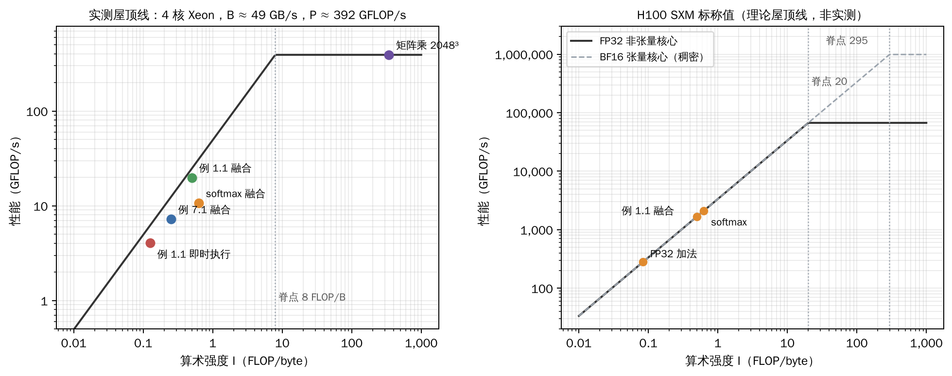
Figure 1.1 The roofline model. Left: the roofline measured on the 4-core CPU used in 第 Section 13, with bandwidth and arithmetic throughput taken as the best of several measurements per Proposition 13.1; the dots are several kernels measured in 第 Section 13. Right: the nominal roofline of the H100 SXM, with BF16 tensor cores shown as dashed lines. Pointwise and reduction operations both have arithmetic intensities below 1 FLOP/byte and lie on the sloped segments of both plots.
In the left plot of Figure 1.1, both the immediate execution and the fused execution of Example 1.1 sit not far below the slope, reaching 65% to 80% of the bandwidth limit: the difference between the two is mainly the number of bytes that have to be moved. 第 Section 13gives the concrete numbers and decomposes the speedup into a ratio of bytes and a ratio of bandwidth efficiency (Proposition 13.3).
Example 1.1 Let
import tensorplay as tp

def f(x, w):
    return (tp.relu(x + w) * 2).sum(-1)

x = tp.randn(64, 128)
w = tp.randn(64, 128)
cf = tp.compile(f, strict_native=True)
y = cf(x, w)
Suppose $x$ and $w$ each contain $N$ float32 elements. Under immediate (eager) execution, f launches four kernels in sequence, add, relu, mul, and sum, producing three intermediate tensors with the same shape as the inputs. The read and write volumes of each kernel are given in Table 1.1.
Table 1.1 Memory traffic of Example 1.1 under immediate execution (in elements)
| Kernel | Read | Write |
|---|---|---|
| add | $2N$ | $N$ |
| relu | $N$ | $N$ |
| mul | $N$ | $N$ |
| sum | $N$ | $N/128$ |
| Total | $5N$ | $3N + N/128$ |
The total memory traffic is about $8N$ elements, that is, $32N$ bytes; the floating-point operation count is about $4N$, giving an arithmetic intensity of about $0.125$ FLOP/byte. If the four operators are fused into a single kernel, it suffices to read $x$ and $w$ once each and write out $N/128$ results, so the memory traffic is about $2N$ elements, that is, $8N$ bytes, and the arithmetic intensity rises to about $0.5$ FLOP/byte. The fused kernel is still memory-bound, but its memory traffic drops to one quarter of the original, and under a bandwidth limit its execution time drops to roughly one quarter as well. The payoff of operator fusion comes precisely from eliminating the round trips of the intermediate tensors to main memory.
The $2N$ above is not accidental; it is a special case of a general law.
Proposition 1.1 (Memory Traffic Lower Bound) Let the set of external inputs of a computation region be $\mathcal I$, and the set of external outputs be $\mathcal O$. Assume: (1) every output element depends on some input elements, and every input element is depended upon by at least one output element; (2) at the start of the region the inputs reside only in main memory, and at the end the outputs must all reside in main memory; (3) on-chip storage is initially empty. Then the amount of traffic between any implementation and main memory satisfies
$$Q \ge \sum_{v\in\mathcal I} b(v) + \sum_{v\in\mathcal O} b(v).$$If on-chip storage is sufficient to hold all the intermediate values needed to compute each output element, then an implementation that fuses the entire region into one kernel, reads each input element exactly once, and writes out no intermediate value attains this lower bound.
Proof By assumptions (1) and (3), the value of every input element must enter on-chip from main memory at least once, or the outputs depending on it cannot be computed, so the read traffic is at least $\sum_{v\in\mathcal I} b(v)$; by assumption (2), every output element is written at least once. The two parts of traffic have different directions and cannot cancel each other, which yields the lower bound. For attainability: if all intermediate values stay on-chip, then main-memory traffic consists only of reading the inputs and writing back the outputs, one element each, which is exactly the lower bound. $\square$
Assumption (1) rules out regions that “read only part of the inputs”, for instance a slice that reads only the first row; the lower bound for such a region should be computed over the elements that are actually depended upon. The on-chip capacity condition needed for attainability holds trivially for pointwise operations; for an operation that reduces and then broadcasts back to the original shape (Example 7.1), all elements of a row must remain on-chip until the row sum is computed, and when the row is long the condition no longer holds — this is exactly the situation that the materialization decisions of Section 6.6are about.
Proposition 1.1 describes the ceiling of fusion: it compresses memory traffic down to the sum of inputs and outputs, after which further speedup can only come from raising bandwidth utilization and no longer from reducing the byte count. It also describes the limitation of fusion: on-chip storage is finite, so if an intermediate value must be used again by a computation far away (for instance a broadcast after a reduction), or must be handed to an external kernel that cannot be fused (for instance a matrix multiplication), then it must be written back to main memory. The materialization and fusion discussed in Sections 6 and 7 approach this lower bound precisely under this limitation.
The parameter strict_native=True requires that compilation raise an error on failure rather than falling back to immediate execution. The CPU kernel that Stax generates for Example 1.1 is given in Listing 1.1.
Listing 1.1 The fused kernel of Example 1.1 (CPU)
#pragma omp parallel for
for (int64_t x0 = 0; x0 < 64; x0 += 1) {
    auto acc = Vectorized<float>(0);
    for (int64_t x1 = 0; x1 < 128; x1 += 16) {
        auto tmp0 = Vectorized<float>::loadu(in_ptr0 + 128*x0 + x1, 16);   // x
        auto tmp1 = Vectorized<float>::loadu(in_ptr1 + 128*x0 + x1, 16);   // w
        auto tmp2 = tmp0 + tmp1;                                     // add
        auto tmp3 = clamp_min(tmp2, decltype(tmp2)(0));              // relu
        auto tmp6 = tmp3 * Vectorized<float>(2.0f);                  // mul
        acc = acc + tmp6;                                            // sum
    }
    out_ptr0[x0] = vec_reduce_all(add, acc);
}
The four operators are merged into one double loop. The outer 64 rows are executed in parallel by OpenMP; the inner loop processes 16 floats at a time, corresponding to the width of an AVX-512 vector register. The addition, the clamp (relu), the multiplication, and the accumulation all take place in registers, one result is written back per row, and none of the three intermediate tensors is allocated. Compared with the result of immediate execution, the maximum absolute error is $1.5\times10^{-5}$, which is a floating-point rounding difference caused by a different order of accumulation (Section 6.5).
When the same function targets a CUDA device, Stax generates the Triton kernel in Listing 1.2.
Listing 1.2 The fused kernel of Example 1.1 (GPU, Triton; import statements and decorator arguments omitted)
@triton_heuristics.persistent_reduction(size_hints={'x': 64, 'r0_': 128}, ...)
@triton.jit
def triton_per_fused_0(in_ptr0, in_ptr1, out_ptr0, xnumel, r0_numel, XBLOCK : tl.constexpr):
    xnumel = 64
    r0_numel = 128
    R0_BLOCK: tl.constexpr = 128
    xoffset = tl.program_id(0) * XBLOCK                      # 本实例负责的起始行
    xindex = xoffset + tl.arange(0, XBLOCK)[:, None]         # 行下标向量  [XBLOCK, 1]
    xmask = xindex < xnumel
    r0_index = tl.arange(0, R0_BLOCK)[None, :]               # 列下标向量  [1, 128]
    r0_1 = r0_index
    x0 = xindex
    tmp0 = tl.load(in_ptr0 + (r0_1 + 128*x0), xmask, eviction_policy='evict_first', other=0.0)   # x
    tmp1 = tl.load(in_ptr1 + (r0_1 + 128*x0), xmask, eviction_policy='evict_first', other=0.0)   # w
    tmp2 = (tmp0 + tmp1)                                                                          # add
    tmp3 = tl.full([1, 1], 0, tl.int32)
    tmp4 = tl.maximum(tmp3, tmp2, tl.PropagateNan.ALL)                                            # relu
    tmp5 = tl.full([1, 1], 2.0, tl.float32)
    tmp6 = (tmp4 * tmp5)                                                                          # mul
    tmp7 = tl.broadcast_to(tmp6, [XBLOCK, R0_BLOCK])
    tmp9 = tl.where(xmask, tmp7, 0)
    tmp10 = tl.sum(tmp9, 1)[:, None].to(tl.float32)                                               # sum
    tl.store(out_ptr0 + (x0), tmp10, xmask)
The two listings come from the same loop-level description (Section 6.3), with operators and statements in one-to-one correspondence: add, relu, mul, and sum correspond in order to tmp2, tmp3, tmp6, and acc in C++, and to tmp2, tmp4, tmp6, and tmp10 here. The difference lies in how the parallelism is organized. The CPU kernel distributes the outer 64 rows with OpenMP, and the inner loop processes one 16-wide vector at a time; the GPU kernel has no explicit loop, and each program instance processes XBLOCK rows at once in a two-dimensional block of [XBLOCK, 128], with several instances in the grid covering all 64 rows. xmask masks off the part of the last block that exceeds 64 rows, and the reduction dimension is exactly 128, so no mask is needed there. 第 Section 9explains this kernel segment by segment.
1.2 The Overall Structure of the Compiler Stack
Figure 1.2 gives the overall structure of the Stax compiler stack.
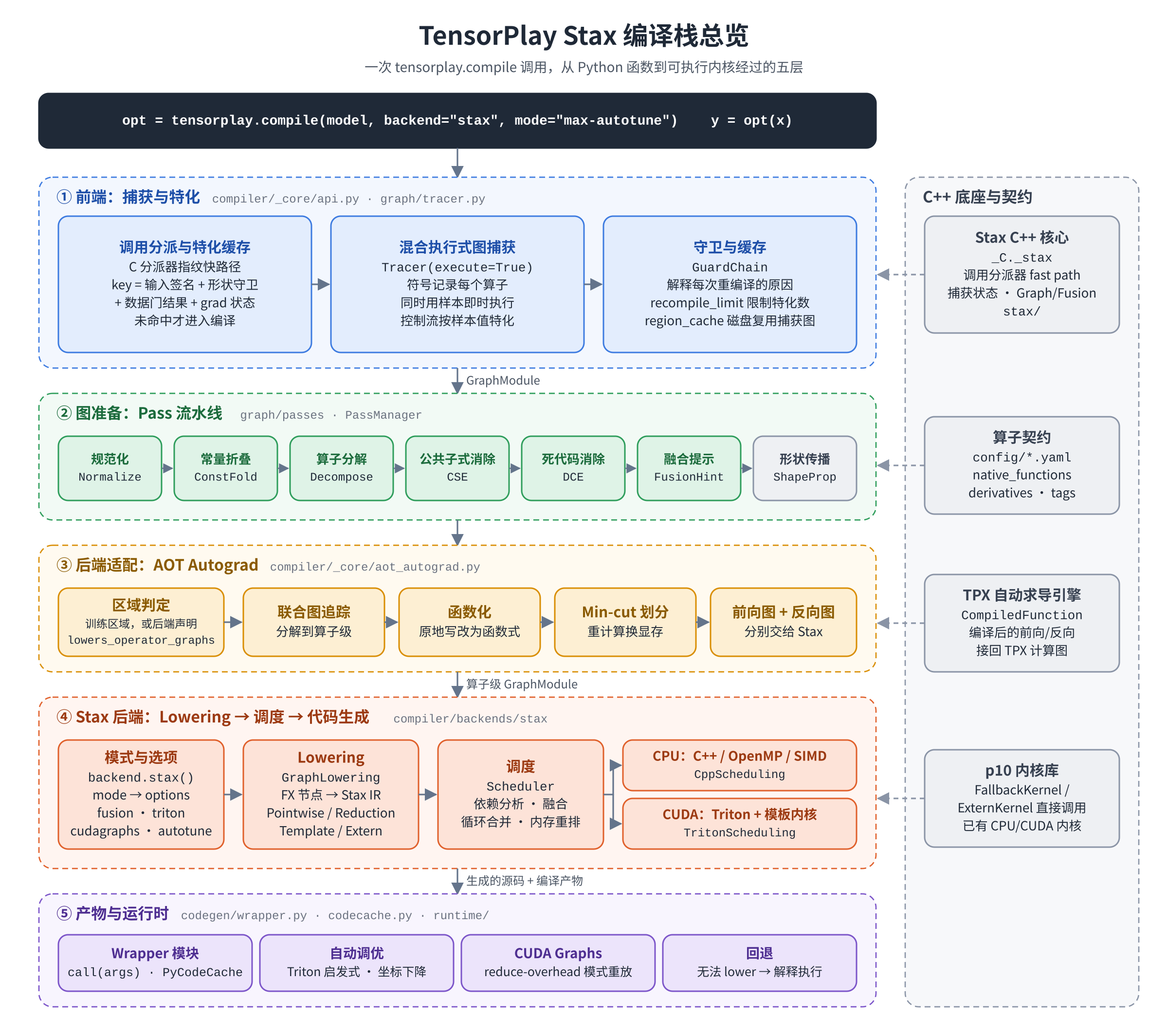
Figure 1.2 The overall structure of the Stax compiler stack. On the left is the main flow on the Python side; on the right are the C++ components it depends on: the call dispatcher, the operator definitions (yaml files under the config directory), the TPX automatic differentiation engine, and the p10 kernel library.
The interface contract between the front end and the back end is
backend(graph_module, example_inputs, **options) -> callable
that is, the back end receives only a captured GraphModule and a set of sample inputs, and returns a callable object. All Python control flow is handled by the front end, so the back end need not be aware of it. Stax is the default back end registered on this interface, and back ends such as TVM, ONNX Runtime, and CUDA Graphs are plugged in the same way. This contract allows the capture strategy of the front end and the implementation of the back end to be replaced independently: the same capture result can be handed to different back ends for comparison, and the same back end can receive graphs produced by different front ends.
1.3 The Layers of Intermediate Representation
A single compilation passes through five program representations in order; each layer solves one class of problems and hands a more concrete description to the layer below. Table 1.2 lists the representation of each layer, the principal decisions made there, and the corresponding chapters.
Table 1.2 The intermediate representations of the Stax compiler stack
| Layer | Program representation | Principal decisions made in this layer | Chapter |
|---|---|---|---|
| Call | Python function and specialization cache | Which already-compiled version to use, whether recompilation is needed | 2 |
| Capture | Python-level GraphModule (nodes are Python calls) | The direction of control flow, which values read data | 3, 4 |
| Operator | Operator-level GraphModule (nodes are operator overloads) | The forward/backward split, which activations to save | 5 |
| Loop | Loop-level intermediate representation (Pointwise, Reduction, ComputedBuffer) | Which values are written to memory, how reductions are split, how views are addressed | 6 |
| Kernel | Schedule nodes and kernel source, wrapper functions | Which loops are merged into one kernel, how to tile, parallelize, and allocate memory | 7 to 9 |
The lower the layer, the closer the representation is to the machine and the more specific the optimizations that can be made, but the less visible program structure remains. For example, at the capture layer F.gelu is a node; at the operator layer it is an operator overload; at the loop layer it has already become a function composed of several ops calls and no longer has a boundary with its neighboring pointwise operations. One of the design points of a compiler is to let each decision be made at the layer where exactly enough information is available.
1.4 Notation
This chapter uses the following notation. $N$ denotes the number of elements of a tensor, and $b(v)$ the number of bytes of a value $v$. $R$ denotes an iteration range (a pointwise dimension), and $R_r$ a reduction range. $\mathbb V$ denotes the set of scalar values. In code, x0 and x1 are loop indices of the pointwise dimensions, r0_ is the index of the reduction dimension, and xindex, yindex, and r0_index in Triton kernels are index vectors for the corresponding dimensions. XBLOCK, YBLOCK, and R0_BLOCK are the tiling sizes of the respective dimensions. The layout of a tensor is described by two tuples, size and stride, and the offset of element $(i_0, \dots, i_{k-1})$ is $\sum_j i_j \cdot \mathrm{stride}_j$.
The statements in this chapter fall into three categories. Theorems and propositions are mathematical conclusions that hold independently of any concrete implementation, and come with proofs; those quoted from the literature are labelled as theorems with their source given. Properties are statements about how Stax is constructed, for example “lowering rules implement fusion by function composition”; their validity depends on how the code is written, and what is given is a reason read off the implementation rather than a proof, so they must be re-checked whenever the code changes. Algorithms and heuristic rules describe what Stax actually does; they generally carry no optimality guarantee, and the text says which optimization problem the rule approximates.
The measurements in this chapter (第 Section 13) were taken with the CPU build of the TensorPlay development branch on a 4-core Intel Xeon (AVX-512, 2.8 GHz), and the generated code in the listings also comes from the development branch. The conclusions on GPU (第 Section 9) and on dynamic shapes (第 Section 10) are based on the source code and the tests, and have no corresponding measured data.
2 Specialization and Caching
2.1 Just-in-Time Compilation as Program Specialization
The behavior of a Python function can depend on any property of its arguments: shape, dtype, the value of scalar parameters, even the data inside tensors. A compiler cannot generate the same efficient code for all inputs; what it does is program specialization: on one concrete input it determines the quantities that affect the structure of the program, treats them as constants, and generates code that is valid only for inputs where “these quantities take the same values”. This is the idea of partial evaluation [2]: the inputs of the program are divided into a static part and a dynamic part, the static part is evaluated ahead of time, and what is obtained is a residual program that accepts only the dynamic part. What characterizes just-in-time compilation is that the static part is not declared by the programmer in advance, but observed by the compiler at the first call.
To state this idea, let the function being compiled be $f: X \to Y$.
Definition 2.1 (Specialization Key and Specialization Version) Call the map $\kappa: X \to \mathcal K$ the specialization key function, and $\kappa(x)$ the specialization key of the input $x$. The program $f_{x_0}$ obtained by capturing and compiling with the input $x_0$ is called a specialization version. If for every $x$ satisfying $\kappa(x) = \kappa(x_0)$ we have $f_{x_0}(x) = f(x)$, then this specialization is said to be sound.
The map $\kappa$ induces an equivalence relation on the input set $X$, and every equivalence class shares one specialization version. The finer $\kappa$ is, the smaller the equivalence classes, the more quantities can be treated as constants, and the more specialized the generated code — but the more specialization versions are needed. The coarser $\kappa$ is, the fewer versions there are, but the less information the compiler can exploit. The design of the specialization key is therefore to choose, between the two, the coarsest partition that keeps the specialization sound.
Which $\kappa$ guarantees correctness? The program obtained by tracing records only tensor operations; every quantity that was used as a constant during tracing must enter the key.
Proposition 2.1 Suppose that when tracing $f$ with $x_0$, the execution path and the generated computation graph depend on the input in only two ways: (1) tensor operations recorded as nodes of the graph; and (2) finitely many quantities $q_1(x), \dots, q_m(x)$ whose values were used as constants during tracing. If $\kappa(x)$ determines $(q_1(x), \dots, q_m(x))$, that is, if $\kappa(x) = \kappa(x_0)$ implies $q_i(x) = q_i(x_0)$ for every $i$, then the specialization is sound.
Proof Assume $\kappa(x) = \kappa(x_0)$. When $f$ is re-executed with $x$, every Python-level predicate and constant is the same as during tracing, so the execution path is the same and the sequence of tensor operations executed is the same as the sequence recorded in the graph. Every node of the graph applies the same operation to a tensor computed from $x$, so $f_{x_0}(x)$ and $f(x)$ agree node by node. $\square$
Proposition 2.1 reduces correctness to a recognition problem: the compiler must find all the $q_i$. 第 Section 3will show that run-time tracing can intercept each $q_i$ at the place where it is used: shape reads, scalar parameters, data-dependent branch predicates, and operations that convert a tensor into a Python scalar.
2.2 The Composition of the Specialization Key
The specialization key of Stax is a four-tuple.
Definition 2.2 (Specialization Key) For a single call, the specialization key is
$$\kappa(x) = (\sigma,\ \gamma_s,\ \gamma_g,\ \rho),$$where $\sigma$ is the input signature; $\gamma_s$ is the shape component, that is, the exact shapes of the arguments whose shapes were read during tracing; $\gamma_g$ is the data gate component, that is, the results of re-evaluating on the current input each predicate that was decided by data value during tracing; and $\rho$ is the current gradient mode.
The input signature $\sigma$ recursively maps each argument, according to its type, into a comparable tuple:
- A tensor maps to (type, shape, dtype, device, requires_grad, strides). In dynamic-shape mode, the shape entry keeps only the rank and the strides entry is rewritten as an expression in terms of the size of each dimension (see below);
None, booleans, integers, floats, and strings map to (type, value), that is, they are specialized by value;- Tuples, lists, and dictionaries map recursively over their elements;
- All other objects map to (type, object identity).
Referring back to Proposition 2.1 makes the origin of each component clear. The shape and dtype of a tensor determine the output metadata of every operator, and also determine the loop ranges and instructions of the generated kernel, so they enter $\sigma$. Python scalars take part directly in the computation during tracing — for example the k in x * k is written into the kernel as a constant — so they enter $\sigma$ by value. If a scalar varies frequently between calls, it should be wrapped as a 0-dimensional tensor and passed in, so that it becomes an input of the graph rather than a constant, and enters the signature only as metadata.
Strides enter the signature because the generated kernel writes down subscripts using the strides seen during tracing (Section 8.5): two tensors of the same shape but with different strides (for example x and x.t(), where $x$ is square) access different addresses when reading the same subscript $(i, j)$, and so by Proposition 2.1 they belong in different equivalence classes. In concrete-shape mode the signature records the stride tuple directly; x and x.t() receive $(n, 1)$ and $(1, n)$ respectively, and each gets its own compiled artifact.
This approach cannot be carried over unchanged in dynamic-shape mode. The strides of a contiguous tensor vary with the shape (the strides of a shape $(s_0, s_1)$ are $(s_1, 1)$); recording the numeric values directly would force a recompilation at every new size because the strides differ, and dynamic shapes would lose their point. Stax therefore rewrites strides into expressions relative to the size of each dimension: it examines the dimensions in increasing order of stride and records a stride of 1 as the constant 1; if the stride of some dimension happens to equal the stride of the preceding (inner) dimension multiplied by its size, it records “the size of this dimension × the expression for that dimension”; otherwise it records the concrete numeric value. Thus a row-major tensor of any size receives the same expression $(\text{size}_1 \cdot 1,\ 1)$, and its transpose receives $(1,\ \text{size}_0 \cdot 1)$, which differs; the inner stride of the slice x[:, ::2] is 2 and the stride of the expansion expand is 0, and both are recorded numerically. The function _stride_signature (tensorplay/compiler/_core/api.py) implements this rewriting, and the test test/stax/test_compile_strides.py verifies two properties: the four layouts contiguous, transposed, expanded, and sliced each compile once and all of them hit on subsequent calls; and in dynamic mode, square matrices of sizes 4, 6, and 8 together with their transposes generate only two artifacts.
Accompanying this, the stand-in made for an input during tracing also preserves the original layout: the compiler first computes, from the input’s shape, strides, and offset, the extent it covers in storage, copies that segment of storage, and then observes it again with the same strides and offset. If the stand-in were always contiguous, the layout seen during tracing would disagree with the layout of the actual argument at the call site, and the generated subscripts would no longer match the layout of the argument.
In dynamic mode, the exact relations between the sizes and the strides of the dimensions are still checked one by one by the input guards (Section 10.4).
$\gamma_s$ exists because dynamic-shape mode specializes only the rank, whereas a function that reads a shape at the Python level, for example x.shape[0] or len(x), obtains a length that has already entered the computation as a constant and must enter the key by exact value. When the back end supports symbolic capture (as Stax does), shape reads remain symbolic expressions and are no longer written down as constants, and $\gamma_s$ is reduced to the tensor inputs nested inside containers, with the judgment about shapes taken over by shape guards (Section 10.4). $\gamma_g$ corresponds to data-dependent control flow, and its construction is the subject of 第 Section 3. $\rho$ enters the key because when gradient mode is on, the traced region attaches backward computation to the outputs, while when it is off the execution produces outputs that violate the contract, and vice versa.
$\gamma_s$ and $\gamma_g$ cannot be determined before the first compilation, because the compiler does not know in advance whether the function reads shapes or makes data-dependent judgments. Only after the first trace is complete does the compiler learn the structure of the key, and extends it accordingly. The structure of the key is therefore determined by the first trace, and the user need not declare it explicitly.
Example 2.1 Call g(x, k) = x * k once with k = 3 and once with k = 4. The $\sigma$ of the two calls differs in the value entry of the second argument, producing two specialization versions. If instead tp.tensor(3.0) and tp.tensor(4.0) are passed in, the signatures of the two calls are the same and only one version is produced; the value of k is read from the tensor at run time.
2.3 Guards
Before a specialization version is invoked, it must be confirmed that the current input belongs to its equivalence class. The predicates that check this condition one by one are called guards.
Definition 2.3 (Guard) Suppose the specialization key can be written as a tuple of components $\kappa(x) = (\kappa_1(x), \dots, \kappa_n(x))$, where each $\kappa_i$ corresponds to a position in the signature structure. The guard of the specialization version $f_{x_0}$ is the family of predicates
$$g_i(x):\ \kappa_i(x) = \kappa_i(x_0),\qquad i = 1, \dots, n.$$
It follows directly from the definition that all the guards hold simultaneously if and only if $\kappa(x) = \kappa(x_0)$. This construction is what it means for the guards to be a projection of the key. It has one practical corollary.
Corollary 2.1 (Explainability) If an input $x$ misses on every specialization version, then for each version there exists at least one $i$ such that $g_i(x)$ does not hold, and the guards that fail point exactly at the components where $\kappa(x)$ differs from that version’s key.
Proof By Definition 2.3, a version $f_{x_j}$ is hit if and only if all of its guards hold, that is, if and only if $\kappa(x) = \kappa(x_j)$. Missing means $\kappa(x) \ne \kappa(x_j)$; two tuples are unequal if and only if there is a component $i$ with $\kappa_i(x) \ne \kappa_i(x_j)$, which is exactly the statement that $g_i(x)$ fails. Thus for each version the set of failing guards equals the set of differing components, and it is non-empty. $\square$
If guards and keys are maintained separately, the two can become inconsistent: the key may already differ while all the guards hold, or the keys may agree while some guard fails, in which case the compiler can neither explain why it is recompiling nor safely reuse a version. Constructing the guards as a projection makes this kind of inconsistency structurally impossible. Each guard in Stax records its path in the signature structure, its condition expression, its expected value, and its actual value; with recompilation logging turned on, every recompilation prints out the guards that failed (Example 3.2).
2.4 Dispatch
Every call has to compute the specialization key and look it up in the cache, and this overhead must be far smaller than the execution time of the kernel itself. Stax divides the decision into three levels ordered by cost, from lowest to highest, as shown in Algorithm 2.1.
Algorithm 2.1 Call Dispatch
输入:实参 args、kwargs
输出:调用结果
1  if 张量对象与上次相同、版本号未变、无 kwargs、梯度模式未变、区域无数据门:
2      return 上次的编译产物(args)                     # 第一级:C 层
3  fp ← 各参数的指纹(张量取对象身份与版本号,标量取值)
4  if fp = 上次的指纹: (σ, γs, γg) ← 上次的键分量      # 第二级:指纹
5  else:               (σ, γs, γg) ← 计算签名与形状分量,重放数据门
6  K ← (σ, γs, γg, ρ)
7  fn ← cache[K]                                        # 第三级:特化缓存
8  if fn 不存在:
9      对每个已有版本检验守卫,记录不成立者
10     fn ← 编译(args, kwargs);cache[K] ← fn
11 记录 fn 为下一次调用的第一级入口
12 return fn(args)
The condition of the first level is strictly stronger than comparing the key: it requires the arguments to be the very same objects, and not merely to have the same key. It suffices to check only object identity and the version counter because the metadata of a tensor does not change during the lifetime of the object, and any in-place modification of the data increments the version counter; when the region has no data gates, tensors of the same object and the same version necessarily have the same specialization key. This level is suited to scenarios that repeatedly call with the same set of buffers. Input batches and parameters in training change continuously, so calls usually go through the second or third level.
The number of specialization versions has an upper bound (8 by default), and the total number of compilations has a separate upper bound (256 by default). The former prevents the cache from growing without bound; the latter prevents repeated compilation in programs whose key keeps changing. Reaching these bounds usually means the key is too fine, and one should check whether there are scalars specialized by value (Section 2.2) or consumptions of values (Section 3.6) that can be rewritten.
2.5 Lifting Free Variables
A function often accesses tensors through global variables, closures, or module attributes; the typical case is model parameters. These tensors are not in the argument list, yet they are read only at each call: between two calls they may be modified in place, and the name may be rebound to a different tensor. If tracing treated them as constants and wrote them into the compiled artifact, subsequent calls would read stale values, violating the premise of Proposition 2.1.
The remedy is to rewrite free variables into explicit arguments, a transformation called lambda lifting in the compilation of functional languages [3]. Stax collects from the bytecode of the function the names that are read as globals and are currently bound to tensors, walks the closure cells and the modules reachable from the function to collect the tensors, arguments, and buffers among them, and then constructs a new function whose arguments are these free tensors together with the original ones. On every call the wrapper reads the current values of these tensors from their original locations and passes them in as leading arguments. After lifting, all of the function’s dependencies on external state appear explicitly in the arguments, and the specialization key together with the version check in the first dispatch level thereby covers them as well.
Example 2.2 Let
scale = tp.ones(128)

def f(x):
    return x * scale

cf = tp.compile(f)
cf(x)
scale.mul_(2)      # 原地修改
cf(x)              # 结果反映修改后的 scale
scale is lifted into an argument. On the second call the version counter of scale has already changed, so the first-level test does not hold; the wrapper reads the current value of scale and passes it in, its signature is unchanged, the existing specialization version is hit, and the result reflects the modified value.
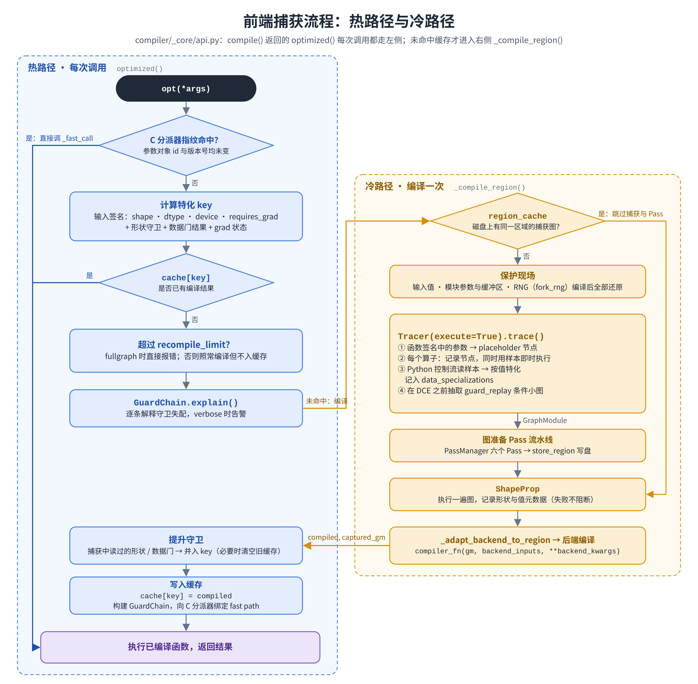
Figure 2.1 The call path. On the left is the dispatch path taken on every call; on the right is the compilation path entered on a cache miss.
3 Graph Capture
3.1 The Computation Graph
The result of capture is a GraphModule: it holds a computation graph and generates from that graph an equivalent piece of Python source code to serve as its forward.
Definition 3.1 (Computation Graph) A computation graph is a directed acyclic graph $G = (V, E)$ together with a total order on $V$. Each node $v \in V$ represents one operation and records its opcode, its target (the name of the called function, method, or attribute), and its arguments; the other nodes appearing among its arguments form the incoming edges $u \to v$, indicating that $v$ uses the value of $u$. The total order must be compatible with the direction of the edges, that is, it is a topological order.
Each node defines exactly one value, and that value never changes after its definition, so a computation graph is a special case of static single assignment (SSA) [4] restricted to programs without control flow. This property makes data dependencies expressible entirely by edges: the users of a value are exactly the endpoints of its outgoing edges, and deciding whether a value can be deleted, can be merged, or can be fused with its users requires examining only the local structure of the graph.
There are six opcodes in total, shown in Table 3.1.
Table Section 3.1 Opcodes of Nodes
| Opcode | Meaning | Target |
|---|---|---|
| placeholder | An input of the function | Argument name |
| get_attr | Read an attribute of the module (parameter, buffer, constant) | Qualified name of the attribute |
| call_function | Call a free function, such as operator.add, tp.relu | The function object |
| call_method | Call a method on a tensor, such as x.sum(-1) | Method name |
| call_module | Call a submodule | Qualified name of the submodule |
| output | The return value of the function | None |
Nodes also carry a metadata dictionary, whose most important entry is val, that is, the value of the node on the sample input (Section 3.3). Subsequent graph transformations rely on it to decide whether the types and shapes agree before and after a rewrite (Section 4.2), and the automatic differentiation layer relies on it to estimate the number of bytes of a tensor (Section 5.3).
The capture result for Example 1.1 is shown in Listing 3.1.
Listing 3.1 The captured graph of Example 1.1
graph(
    %x : [num_users=1] = placeholder[target=x]
    %w : [num_users=1] = placeholder[target=w]
    %add shape=(64, 128) : [num_users=1] = call_function[target=operator.add](args = (%x, %w), kwargs = {})
    %relu shape=(64, 128) : [num_users=1] = call_function[target=tensorplay.functional.relu](args = (%add,), kwargs = {})
    %mul shape=(64, 128) : [num_users=1] = call_function[target=operator.mul](args = (%relu, 2), kwargs = {})
    %sum_0 shape=(64,) : [num_users=1] = call_method[target=sum](args = (%mul, -1), kwargs = {})
    return sum_0
)
The nodes in the captured graph are still Python-level calls: operator.add corresponds to the + in the source, and sum is a tensor method call. This level involves neither operator overloads nor dispatch; 第 Section 5is what rewrites it into an operator-level graph.
3.2 Proxy Tracing
There are two ways to construct a computation graph: analyze the source or the bytecode of the program, or execute the program and record what it did. TensorPlay takes the latter, that is, tracing. The result of tracing is a straight-line program obtained by unrolling the program along one execution path: loops are unrolled, function calls are inlined, and only the side of a branch that was actually taken is retained.
Tracing is implemented through operator overloading, the same technique used by operator-overloading-based automatic differentiation tools. The tracer creates one placeholder node per argument and calls the user function with proxy objects standing in for the actual arguments. The proxies overload Python’s arithmetic and comparison operators and implement the function dispatch protocol, so that library function calls taking a proxy as an argument, such as tp.relu(p), are intercepted as well. Each interception creates a new node in the graph and returns a new proxy wrapping that node. When the function returns, the proxies contained in the return value are collected into the arguments of the output node.
Tracing by default enters the forward of a submodule and records the tensor operations inside it, rather than recording a single call_module node. Inlining lets the subsequent layers see the complete operator sequence, so fusion can cross module boundaries.
3.3 Run-Time Sampling
A purely symbolic tracing knows only how each value is computed, not what it equals, and therefore cannot answer any question about values posed at the Python level. The TensorPlay tracer runs in a hybrid mode: each time it records a node, it actually executes on the sample input the call that node represents, and saves the result in the metadata val. Every proxy thus carries a symbol (the node in the graph) and a concrete value (the result on the sample) at the same time.
The execution is performed with gradient recording turned off, and no backward graph is constructed for the sample computation. This execution is auxiliary: if a node fails to execute on the sample, that node stays symbolic and the tracing itself is unaffected; an error is raised only when a later piece of control flow actually needs its value.
3.4 Data-Dependent Control Flow
Example 3.1 Let
def f(x):
    if x.sum() > 0:
        return x * 2
    return x - 1
The result of x.sum() > 0 is a proxy, and the if statement calls its __bool__ method, which demands a Python boolean. A purely symbolic tracing cannot proceed here; this is precisely where the symbolic_trace of torch.fx [5] reports an error.
In hybrid mode, __bool__ returns the result on the sample and tracing continues along the corresponding branch. This choice makes the graph obtained by tracing valid only for inputs that “take the same branch”. Borrowing the terminology of symbolic execution [6], the conjunction of all branch conditions collected along one execution path is called the path condition, and the graph obtained by tracing is equivalent to the original program on inputs where the path condition holds.
Definition 3.2 (Data Gate) During tracing, whenever the Python layer derives a concrete value from tensor data and uses it to decide where execution continues, this is called a data gate. Suppose the value of the $k$-th data gate is $c_k = h_k(x)$, where $h_k$ can be computed from the nodes of the graph, and its value at tracing time is $c_k^0 = h_k(x_0)$. The data gate component is defined as
$$\gamma_g(x) = \bigl(h_1(x), \dots, h_m(x)\bigr).$$
Data gates are one of the sources of the second kind of dependency in Proposition 2.1: $c_k$ is used as a constant to determine the execution path, so it must enter the specialization key. Besides __bool__, the proxy has several other entry points that convert tensor values into Python values, handled as shown in Table 3.2.
Table 3.2 Kinds of Data Specialization
| Kind | Trigger | Handling |
|---|---|---|
| bool | if, while, and, or, not | Take the truth value on the sample; record it as a data gate |
| index | Using a tensor as an index or a range, such as x[:n], range(n) | Take the integer value; record it as a data gate |
| int, float | int(t), float(t) | Take the value on the sample as a constant; record it as a data gate (Section 3.6) |
| iter | Iterating over a value whose sample is a non-tensor sequence | Take the contents of the sequence; record it as a data gate |
| Shape read | len(t), t.shape | Recorded as a metadata read; the shape enters $\gamma_s$ |
The difference between a shape read and a data gate is that the shape can be obtained directly from the metadata of the input and requires no computation to be evaluated, whereas the value of a data gate has to be computed from the input data.
3.5 Program Slicing and Guard Replay
The values of the data gates $h_k(x)$ must be recomputed on the real input at every call, in order to decide whether the input falls into the equivalence class of an existing version. Re-executing the entire function is plainly not acceptable; what is needed is only that part of the program which computes the various $h_k$. This is called program slicing [7] in program analysis.
Definition 3.3 (Backwards Slice) In a computation graph $G$, the backward slice of a node set $D$ is the subgraph consisting of the nodes in $D$ and all of their ancestors, that is,
$$\mathrm{slice}(D) = \{\, u \in V \mid \text{存在从 } u \text{ 到某个 } d \in D \text{ 的有向路径} \,\} \cup D.$$
On a directed acyclic graph the backward slice is simply the set reachable from $D$ along incoming edges, and can be obtained by a single graph traversal, as shown in Algorithm 3.1.
Algorithm 3.1 Extraction of the Guard Replay Subgraph
输入:计算图 G,数据门节点集合 D
输出:子图 M,数据门在样例上的取值 c⁰
1  needed ← ∅;pending ← D
2  while pending 非空:
3      n ← pending.pop()
4      if n ∈ needed: continue
5      needed ← needed ∪ {n}
6      将 n 的全部参数节点加入 pending
7  按 G 的拓扑序复制 needed 中的节点,得到 M;M 的输出为 D 中各节点
8  c⁰ ← 各数据门在样例上的取值
9  return M, c⁰
Each node enters needed at most once and each edge is examined at most once, so the running time of the algorithm is $O(|V| + |E|)$. The resulting subgraph $M$ is called the guard replay subgraph; executing $M$ on the real input at every call yields $\gamma_g(x)$.
Does equality of the replayed vector with the traced vector characterize exactly “taking the same path”? The following proposition answers affirmatively.
Proposition 3.1 Suppose the data gates $1, \dots, m$ are encountered in order along the traced path. For any input $x$, $\gamma_g(x) = \gamma_g(x_0)$ if and only if executing $f$ with $x$ passes through the same $m$ data gates in order and each data gate takes the same value as during tracing.
Proof Induct on the index of the data gates. Suppose that when $f$ is executed with $x$, the values of the first $k$ data gates agree with those at tracing time. Then the path up to the $(k+1)$-th data gate is the same as the traced path, so the way $f$ computes the $(k+1)$-th data gate is the same as recorded in the graph and its value equals the $h_{k+1}(x)$ that $M$ computes on $x$. Therefore, if $\gamma_g(x) = \gamma_g(x_0)$, the induction carries through to all $m$ data gates; conversely, if $f$ passes through these data gates in order with the same values on $x$, then every $h_k(x)$ equals the value at tracing time. $\square$
The slice in Proposition 3.1 depends only on the structure of the graph, so the moment at which it is extracted is crucial.
Corollary 3.1 The guard replay subgraph must be extracted before dead code elimination.
Proof The value of a data gate is consumed only by a Python if statement and does not flow to the outputs of the graph. Dead code elimination deletes every node that cannot reach an output (Section 4.6), so it deletes the nodes that compute the data gates. Extracting afterwards leaves those nodes out of the slice, the replay can no longer obtain $\gamma_g(x)$, Proposition 3.1 no longer applies, and the compiled artifact will fail to notice a change of branch. $\square$
Example 3.2 Call the f of Example 3.1 in turn:
cf = tp.compile(f, strict_native=True)
cf(tp.ones(4, 8))         # 输出全为 2
cf(-2 * tp.ones(4, 8))    # 输出全为 -3
cf(tp.ones(6, 8))         # 输出全为 2
All three results are correct, and three specialization versions are ultimately present in the cache. The replay subgraph in this example contains only two nodes, sum and the comparison. With recompilation logging turned on, the printed reason for recompilation is:
recompiling 'f': control-flow gate outcomes match the traced branch
recompiling 'f': inputs[0][0][2][0] == 4; inputs[0][0][2][0] == 4; control-flow gate outcomes match the traced branch
The first line corresponds to the second call: the signature is the same but the value of the data gate differs. The second line corresponds to the third call, which is compared against the two existing versions in turn: compared with the first version the shape differs; compared with the second version both the shape and the data gate differ. This is exactly the explainability stated in Corollary 2.1. The path inputs[0][0][2][0] denotes, in order, the positional-arguments part, the first argument, the shape entry of the tensor signature, and dimension 0 of the shape.
3.6 The Consumption of Values
Operations such as int(x.max()) and float(...) that convert a tensor into a Python scalar are likewise data gates, and even finer than bool data gates: their value space may be large, and every distinct value corresponds to a specialization version. Such conversions cannot return a symbolic value, because CPython requires __int__ and __float__ to return an exact int and float.
If a value only takes part in subsequent tensor operations and does not determine control flow, there is no need to specialize it. tensorplay.graph.gate is used to declare this explicitly: a value declared this way stays a proxy of a 0-dimensional tensor and becomes a run-time input of the graph, and it is frozen only when int() or float() is called explicitly.
Example 3.3 Compare the following two versions:
def f1(x):
    n = int(x.sum())            # 数值进入特化键
    return x * n

def f2(x):
    n = tp.graph.gate(x.sum())  # 数值保持为张量
    return x * n
Call each of an all-ones and an all-twos tensor of shape $2\times3$ once; the two versions give the same result (first elements 6 and 24 respectively), but f1 has two specialization versions and f2 has only one. If if n > 3: then appears inside f2, the truth value of that comparison is still a data gate, but n itself no longer enters the key. In the words of Section 2.1, gate moves a quantity from the static part to the dynamic part.
3.7 Isolating Side Effects
Tracing actually executes the user function. In order that whether compilation happened be unobservable to the caller, the side effects produced by tracing must be isolated:
- If the function modifies an input in place, the input is copied before tracing and restored afterwards, so the input observed by the caller is the same as when it is not compiled;
- Module state (such as the running statistics of a normalization layer) is treated the same way;
- The random number generator is forked before tracing, so the random numbers consumed by the tracing and compilation process do not advance the caller’s generator, and the compiled version and the immediate version therefore produce the same random sequence.
Pure Python side effects, such as printing or appending elements to an external list, do not appear in the computation graph and happen only once, during tracing. This is an inherent property of tracing as a method of graph construction (Section 12.1).
4 Graph Transformation
Before being handed to the back end, the captured graph passes through a set of front-end transformations. The purpose of these transformations is not to generate faster code but to bring the graph into a canonical, lean form, so that the later layers face fewer formulations and fewer nodes. This section first gives the general framework for graph transformation, and then discusses one by one the conditions under which each transformation holds.
4.1 Rewrite Systems and Fixed-Point Iteration
A graph transformation consists of a number of rewrite rules.
Definition 4.1 (Rewrite Rule) A rewrite rule is a pair of graph patterns $l \Rightarrow r$. If some subgraph of the graph $G$ matches $l$ and is replaced by the corresponding instance of $r$, the resulting graph is written $G’$, and $G$ is said to be rewritten into $G’$ in one step. If for every input $x$ we have $\llbracket G’ \rrbracket(x) = \llbracket G \rrbracket(x)$, the rewrite is said to preserve semantics, where $\llbracket G \rrbracket$ denotes the function computed by the graph.
Semantics preservation is required of every rule, and Section 4.2 to Section 4.6discusses them one by one. Besides that, a set of rules must satisfy termination as a whole: rewriting must not proceed indefinitely.
The TensorPlay front end executes six transformations in order: normalization (NormalizeOperators), constant folding (ConstFold), decomposition (DecomposePass), common subexpression elimination (CSE), dead code elimination (DCE), and pointwise region annotation (PointwiseFusionHint); this constitutes one round. If any transformation changes the graph within a round, another round is executed, until some round makes no change at all. In other words, the sequence of transformations is iterated to a fixed point. The iteration is necessary, because the output of one transformation may create new opportunities for the transformations placed before it (Example 4.2).
Proposition 4.1 (Termination) Suppose there exists a measure $\mu$ from graphs to a well-founded set such that every transformation either leaves the graph unchanged or makes $\mu$ strictly decrease. Then the fixed-point iteration terminates after finitely many rounds.
Proof If a round changes the graph, then at least one transformation changes the graph and $\mu$ decreases at least once, while the remaining transformations do not increase $\mu$. There is no infinite descending chain in a well-founded set, so the number of rounds that make changes is finite. $\square$
For the six transformations above, one may take the lexicographic measure
$$\mu(G) = (\text{组合算子节点数},\ \text{节点总数},\ \text{常数位于左侧的二元运算数}).$$Decomposition decreases the first component (the primitives it produces are not decomposed again), even though it increases the total node count; CSE, DCE, and identity elimination decrease the second component; moving constants to the right decreases the third component; region annotation only writes metadata and from the second round on makes no change to the graph. The implementation additionally sets an upper bound of 16 rounds as a safeguard for when the rule set is expanded in the future.
It is worth noting that fixed-point iteration guarantees only termination, not that the result is independent of the order in which the transformations execute. If a rewrite system satisfies confluence, that is, any two rewriting paths can eventually be merged, then the result is unique; a general rule set does not satisfy this property. The order of the transformations is therefore itself part of the design: normalization comes first, so that later patterns have to handle only one formulation; CSE comes after decomposition, so that identical subchains decomposed out of different composite operators can be merged; region annotation comes last, so that what it sees is the final graph.
4.2 Algebraic Identities and Floating-Point Semantics
The normalization transformation applies three kinds of rewrite: in a commutative operation the scalar constant is moved to the right, so 2 * x is rewritten as x * 2; algebraic identities are eliminated, so x * 1 is rewritten as x; an in-place operation with no other users is rewritten into its non-in-place form. The first and the third obviously preserve semantics; the question is concentrated on the identities.
Over the reals, $x + 0 = x$, $x \cdot 1 = x$, and $x \cdot 0 = 0$ are all identities. But the numbers in a tensor are IEEE 754 floating-point numbers [8], whose range contains $\pm 0$, $\pm\infty$ and NaN, and whose operation results must be rounded. Under this semantics, whether an identity holds has to be checked case by case; the results are given in Table 4.1.
Table 4.1 Whether Common Identities Hold under IEEE 754 Semantics
| Rewrite | Holds Exactly | Counterexample or Note |
|---|---|---|
| $x \cdot 1 \Rightarrow x$ | Yes | For every $x$, including $\pm 0$, $\pm\infty$, NaN |
| $x / 1 \Rightarrow x$ | Yes | Same as above |
| $x - 0 \Rightarrow x$ | Yes | $(-0) - (+0) = -0$ |
| $x + 0 \Rightarrow x$ | No | $(-0) + (+0) = +0$; the sign of zero changes |
| $x + (-0) \Rightarrow x$ | Yes | The true identity element of addition is $-0$ |
| $-(-x) \Rightarrow x$ | Yes | Negation only flips the sign bit |
| $x \cdot 0 \Rightarrow 0$ | No | $\infty \cdot 0 = \mathrm{NaN}$, $\mathrm{NaN} \cdot 0 = \mathrm{NaN}$, $(-1) \cdot 0 = -0$ |
| $(x + y) + z \Rightarrow x + (y + z)$ | No | The rounding error depends on the summation order (Section 6.5) |
$x + 0 \Rightarrow x$ differs from the original program only in the sign of zero, and $+0$ and $-0$ compare equal, so they can be distinguished only through $1/x$, copysign, or atan2. Deep learning compilers generally accept this rewrite, and so does TensorPlay. $x \cdot 0 \Rightarrow 0$, on the other hand, turns NaN and infinity into 0 and thus conceals numerical anomalies, so it is excluded. The last row of the table states a more general fact: floating-point arithmetic does not satisfy associativity, so any transformation that changes the order of operations preserves semantics only in an approximate sense — a point that is especially important in the splitting and vectorization of reductions.
Besides the value, the elimination of an identity must also preserve the other attributes of the tensor:
- Type. Adding
0.0to an integer tensor yields a floating-point tensor, sox + 0.0cannot be rewritten asx; - Shape. Broadcasting can make the shape of
x + 0larger than that ofx, for instance when the right-hand side is a zero tensor of shape $4\times1$; - Aliasing. If the rewritten value is an output of the graph while
xis an input of the graph, then after the rewrite the output and the input share storage, and a modification by the caller to one of them affects the other, whereas in the original program they are two different tensors.
The first two points are decided by the sample value in the node metadata, and when the sample value is missing no rewrite is performed; the third point is decided by the structure of the graph.
Example 4.1 Let n(x) = (2 * x + 0).exp(). The graph before and after normalization is as follows (node metadata omitted):
改写前:
    %mul = call_function[target=operator.mul](args = (2, %x))
    %add = call_function[target=operator.add](args = (%mul, 0))
    %exp = call_method[target=exp](args = (%add,))
改写后:
    %mul = call_function[target=operator.mul](args = (%x, 2))
    %exp = call_method[target=exp](args = (%mul,))
The constant 2 is moved to the right and + 0 is eliminated. The result of mul is an intermediate value of the graph rather than an output, and neither its type nor its shape changes, so all three conditions are satisfied.
4.3 Constant Folding
Constant folding evaluates at compile time every operation whose arguments are all constants. TensorPlay folds only arithmetic, comparison, and subscript operations between Python scalars, and leaves tensor operations entirely to the back end. The reason is that folding a tensor operation means embedding its result as a constant in the compiled artifact: if the result is a large tensor, the artifact inflates accordingly, and every call has to read it back from the constant pool, while computing it at run time is often just as fast. Most scalar arithmetic at the Python level has already been evaluated directly by the interpreter during tracing, so this transformation mainly handles the constant expressions newly produced by the other transformations.
4.4 Decomposition of Composite Operators
A composite operator is an operator that can be expressed as a composition of several primitives, such as selu, gelu, and log1p. The payoff of decomposition is that the resulting primitives can be fused with neighboring pointwise operations and that identical subchains can be merged by CSE. But decomposition also has costs.
The first is numerical precision. Take $\log(1+x)$ as an example, and let the unit roundoff be $u$ (in float32, $u = 2^{-24}$). Computing $1 + x$ first gives $\mathrm{fl}(1+x) = (1+x)(1+\delta)$ with $|\delta| \le u$, and taking the logarithm afterwards gives
$$\log \mathrm{fl}(1+x) = \log(1+x) + \log(1+\delta) \approx \log(1+x) + \delta.$$When $|x|$ is very small, $\log(1+x) \approx x$, so the relative error is about $|\delta| / |x|$, which can reach $u/|x|$. Taking $x = 10^{-10}$, the float32 value of $1 + x$ rounds to 1 and the result is 0, a relative error of 100%. The dedicated log1p implementation avoids this catastrophic cancellation and should therefore not be decomposed. The same holds for $e^x - 1$ and for the hyperbolic functions.
The second is storage in automatic differentiation. In the joint graph used for training, every intermediate value produced by decomposition may be read by the backward pass, whereas the dedicated differentiation rule of a composite operator often needs only its inputs (第 Section 5).
The third is that a composite operator is often already a fused kernel in its own right. Decomposition pays off only when the resulting primitives can be fused further with other operations in the graph.
Accordingly, TensorPlay treats composite operators as shown in Table 4.2. The operators left as they are are still expanded into scalar operations in the loop body during the lowering stage of 第 Section 6, and are fused with their neighbors there; not decomposing therefore does not mean giving up fusion, it only defers it to the layer where the numerical implementation is under control.
Table 4.2 Treatment of Composite Operators
| Treatment | Operators |
|---|---|
| Decomposed | selu, relu6, mish, tanhshrink, hardshrink, softshrink, clamp, lerp, addcmul, addcdiv, logit, exp2, square, squared_difference, sec, csc, cot, deg2rad, rad2deg |
| Left as is | silu, gelu, elu, leaky_relu, hardtanh, hardsigmoid, threshold, softplus, log1p, expm1, log10, sinh, cosh, asinh, acosh, atanh |
| Optionally decomposed | softmax, log_softmax, group_norm (not decomposed by default) |
Example 4.2 Let
def s(x):
    y = x * 3
    return F.selu(y) + F.selu(y * 1) * 2
The role of each transformation is as follows (only the transformations that changed the graph are listed, node metadata omitted):
[第 1 轮] NormalizeOperators:y * 1 被消去,两处 selu 的参数都成为 %mul
[第 1 轮] DecomposePass:两处 selu 各展开为一条链
    %exp   = call_method[target=exp](args = (%mul,))
    %sub   = call_function[target=operator.sub](args = (%exp, 1))
    %mul_0 = call_function[target=operator.mul](args = (1.6732632423543772, %sub))
    %gt    = call_function[target=operator.gt](args = (%mul, 0))
    %where = call_function[target=tensorplay.functional.where](args = (%gt, %mul, %mul_0))
    %mul_2 = call_function[target=operator.mul](args = (1.0507009873554805, %where))
    %exp_0 = call_method[target=exp](args = (%mul,))
    ...(第二条链,结构相同)
[第 1 轮] CSEPass:两条链合并为一条,%mul_2 的使用者数变为 2
[第 1 轮] PointwiseFusionHint:全部节点标为同一个逐元素区域
[第 2 轮] NormalizeOperators:分解产生的 1.6732632423543772 * sub 与
          1.0507009873554805 * where 中的常数移至右侧
[第 3 轮] 无改动,迭代结束
This example illustrates the interaction between the transformations: only after normalization eliminates y * 1 do the arguments of the two selu calls coincide, and only then can CSE merge them; the constants produced by decomposition sit on the left and need a second round of normalization to move to the right. In terms of the measure of Proposition 4.1, the decomposition in round 1 lowers the number of composite operators from 2 to 0, CSE lowers the total node count, round 2 lowers the number of left-hand constants, and in round 3 no component changes any further.
4.5 Common Subexpression Elimination
Common subexpression elimination (CSE) merges the nodes that compute the same value. On a computation graph it is equivalent to value numbering in compiler theory: a key is computed for each node (target, representative node of each argument), nodes with the same key compute the same value, the one that appears first is retained, and the users of the remaining nodes are redirected to it.
Proposition 4.2 If the nodes are processed in topological order and the keys already seen are recorded in a hash table, then a single scan merges all syntactically identical nodes, in expected time $O(|V| + |E|)$.
Proof When a node $v$ is processed, its arguments have already been processed and replaced by their respective representatives. If two nodes have the same target and the same representatives for their arguments, their keys are the same and they hit in the hash table; otherwise some argument of theirs computes a different value, or their targets differ, and they should not be merged. Each node computes its key once, and the length of the key is its in-degree, so the total time is proportional to the sum of the node and edge counts. $\square$
The premise of value numbering is that operations are referentially transparent, that is, identical arguments always yield identical results and the operation has no observable side effects. Random operators (dropout, randn, and the like) violate the former, since two calls give different results; in-place operators (add_, mul_, and the like) violate the latter, since the effects of two modifications accumulate. Both kinds are excluded from CSE. CSE also does not recognize commutativity: x + y and y + x can be merged only after normalization has unified the formulation, which is another reason why normalization must precede CSE.
4.6 Dead Code Elimination
A node whose value cannot reach any output is called dead code, because deleting it does not change the function the graph computes. On a directed acyclic graph, the set of live nodes is exactly the set reachable from the output nodes along incoming edges, that is, the backward slice of the output node set (Definition 3.3). DCE computes this set and deletes the remaining nodes, in $O(|V| + |E|)$ time.
Input nodes are always retained, even when unused, because deleting one would change the calling convention of the function. Moreover, nodes with side effects must be retained regardless of whether their values are used. Corollary 3.1 is derived precisely from this definition of DCE: the computation of a data gate cannot reach an output, and so in the eyes of DCE it is dead code.
4.7 Annotating Pointwise Regions
The last transformation identifies the maximal pointwise regions in the graph and writes a region number into the nodes inside each region. Let the fusible pointwise operators form a node subset $P \subseteq V$; the region sought is the connected components, with edge directions ignored, of the subgraph induced by $P$. The algorithm uses a union-find structure: every node in $P$ starts as its own set, and for every edge whose two endpoints lie in $P$ the sets of the endpoints are merged. With path compression and union by rank, the total time is $O\bigl((|V| + |E|),\alpha(|V|)\bigr)$, where $\alpha$ is the inverse Ackermann function.
The annotation for Example 1.1 is
[('add', 'pointwise', 0), ('relu', 'pointwise', 0), ('mul', 'pointwise', 0), ('sum_0', None, None)]
add, relu, and mul form region 0; sum is not a pointwise operator and lies outside the region. This annotation is used by back ends that need fusion information. Stax judges fusion separately on the loop-level intermediate representation (Sections 6 and 7), and can bring reductions into the scope of fusion as well, which connected components at the graph level cannot express.
4.8 Operator-Level Decomposition
The decomposition of Section 4.4acts on the Python-level graph and is keyed by method name or function name, with the goal of expanding composite operators into fusible primitives. After the graph enters the automatic differentiation layer it is traced once more at the dispatcher level (Section 5.1); at that point every call has landed on a definite operator overload, and decomposition can therefore be carried out at the operator level. TensorPlay maintains an operator-level decomposition table with about five hundred rules, covering operators for normalization, loss functions, padding, interpolation, the backward of activation functions, and more. Whenever tracing meets an operator overload, the dispatcher first consults this table: if a rule exists, the rule is executed instead of the operator itself, and what is recorded is the individual operators produced by expanding the rule.
The decomposition table does not take effect in its entirety. For a given back end, operators fall into two classes.
Definition 4.2 (The Basis of a Back End) Call a set of operators $\mathcal B$ the basis of a back end if every operator in $\mathcal B$ has an implementation of its own in that back end, that is, a lowering rule (第 Section 6), a template, or a library call.
Stax constructs the decomposition set actually used from the decomposition table and the basis: an operator is decomposed only if it does not belong to $\mathcal B$ and does not produce random numbers. Operators in $\mathcal B$ are left as they are and handed to the back end for implementation in a dedicated way; operators that produce random numbers are also left as they are, because a random operator is not referentially transparent (Section 4.5), and after expansion the way the parts consume the random state must be guaranteed consistent by other means.
Proposition 4.3 Define the depth $d(o)$ of each operator $o$ as follows: $d(o) = 0$ if $o \in \mathcal B$ or $o$ has no decomposition rule; otherwise $d(o)$ is one larger than the maximum depth of the operators on the right-hand side of its rule. If the depth is defined for every operator (that is, if there are no cyclic references among the rules), then recursive decomposition terminates in finitely many steps, and every operator in the result either belongs to $\mathcal B$ or has no decomposition rule.
Proof Induct on $d(o)$. When $d(o) = 0$, $o$ is not decomposed. When $d(o) = k > 0$, $o$ is replaced by finitely many operators of depth less than $k$, and by the induction hypothesis each of them is fully decomposed in finitely many steps. $\square$
An operator with no decomposition rule and not belonging to $\mathcal B$ becomes a fallback kernel (Section 6.1) and is executed as is by the framework. Proposition 4.3 and Proposition 4.1 are the same kind of argument: the measure of the former is depth, and the measure of the latter is the lexicographic triple.
Why are operators belonging to $\mathcal B$ not decomposed? Take variance and mean as an example. The decomposition table writes var_mean as first computing the mean and then the mean of the squared deviations, which after lowering becomes two reductions; Stax’s lowering rule instead uses the Welford formulation of Section 6.5to compute both in a single fused reduction, halving the memory traffic and numerically avoiding the cancellation of the $\sum x^2 - n\bar x^2$ form. The same holds for the backward of layer_norm, of softmax, and of gelu. Decomposition is a fallback when a dedicated implementation is missing, not a first choice.
Example 4.3 Compile F.layer_norm(x, (8,), w, b) and F.mse_loss(x, y) separately; the operator-level graphs handed to Stax are as follows (metadata omitted):
layer_norm:
    native_layer_norm = tp.native_layer_norm.default(primals_1, [8], primals_2, primals_3, 1e-05)
    getitem = getitem(native_layer_norm, 0)
mse_loss:
    sub  = tp.sub.Tensor(primals_1, primals_2)
    mul  = tp.mul.Tensor(sub, sub)
    mean = tp.mean.default(mul)
native_layer_norm belongs to the basis and is retained as it is; mse_loss has no lowering rule and is decomposed into the three primitives subtraction, multiplication, and mean, after which they can be fused into a single reduction kernel.
4.9 Functionalization
All of the preceding transformations assume that the graph is a pure function: each node is uniquely determined by its arguments and modifies no existing value. A user program, however, may contain in-place modifications such as x.mul_(2), and in-place modifications of views, such as y[0].add_(1), which modifies row 0 of y. In-place modification invalidates the premises of value numbering and dead code elimination: the same name denotes different values at different moments, and deleting an in-place operation whose “result is unused” would change the behavior of the program.
Definition 4.3 (Functionalization) Rewriting a graph that contains in-place modifications into an equivalent graph that contains none is called functionalization. After the rewrite, each in-place modification produces a new value, and every subsequent use of the original value is changed into a use of the new value; if what is modified is an input of the graph, a single copy writes the final value back into the input at the end of the graph.
Functionalization and SSA construction [4] are the same idea generalized to storage: SSA introduces a new name for every assignment, and functionalization introduces a new value for every modification of a tensor. The difficulty lies in views. A modification of the view $v = \mathrm{view}(b)$ actually modifies part of $b$, so functionalization must at the same time produce a new value for $b$. Suppose the view operation $\mathrm{view}$ has a “scattering inverse” $\mathrm{scatter}(b, v’)$, which returns a tensor equal to $b$ except that at the positions covered by the view it takes the values of $v’$. Then a modification of the view $v \leftarrow g(v)$ can be rewritten as
$$v' = g(\mathrm{view}(b)),\qquad b' = \mathrm{scatter}(b, v').$$Proposition 4.4 Suppose the view operation and its scattering inverse satisfy $\mathrm{view}(\mathrm{scatter}(b, v’)) = v’$, and $\mathrm{scatter}(b, v’)$ agrees with $b$ at the positions not covered by the view. Then after rewriting an in-place modification of the view as above, $b’$ is elementwise identical to the contents of $b$ after the original program executes the modification.
Proof In the original program, the positions covered by the view are written with the result of $g$ applied to the original contents, that is, with the corresponding elements of $v’$, and the remaining positions are unchanged. $b’$ takes $v’$ at the positions covered by the view and $b$ at the remaining positions, so the two agree. $\square$
Slices, selects, transposes, and other views all have such a scattering inverse; for example the selection select corresponds to select_scatter. An in-place operator with no functional overload cannot be rewritten this way, in which case it is wrapped as a whole into a node that records which argument it modifies; before lowering, Stax expands such a node into the form “copy the modified argument, then execute in place on the copy”.
Example 4.4 Let
def f(x, y):
    x.mul_(2)
    y[0].add_(1)
    return x + y
The operator-level graph after functionalization is (metadata omitted):
mul            = tp.mul.Scalar(primals_1, 2)
select         = tp.select.int(primals_2, 0, 0)
add            = tp.add.Scalar(select, 1, 1)
select_scatter = tp.select_scatter.default(primals_2, add, 0, 0)
add_0          = tp.add.Tensor(mul, select_scatter)
copy_          = tp.copy_.default(primals_1, mul)
copy__0        = tp.copy_.default(primals_2, select_scatter)
return (add_0,)
x.mul_(2) becomes the functional mul, and every subsequent use of x is changed into a use of mul. y[0].add_(1) becomes three steps: taking the view select, computing add on it, and then obtaining the new value of y with the scattering inverse select_scatter. The two copy_ at the end write the new values back into the inputs, so that the side effects observed by the caller agree with those of immediate execution. The body of the graph is now a pure function, and the transformations of Section 4.5 and Section 4.6can be applied to it safely.
The cost of functionalization is that copies may be added: a modification performed in place in the original program needs a new block of storage after functionalization. This cost is recovered at the scheduling stage: if a buffer is no longer used after being read by some kernel, and that kernel’s output has the same size, type, and subscripts as the buffer, then the kernel can write its result directly into that buffer (Section 7.5). Functionalization and in-place reuse are therefore a pair of inverse transformations: the former removes in-place modification for the convenience of analysis, and the latter restores it once the analysis is complete.
4.10 The Full Picture of the Transformations
At this point all the graph transformations on the compilation path can be listed by layer, as shown in Table 4.3.
Table 4.3 Graph Transformations on the Compilation Path
| Layer | Transformation | Effect | Section |
|---|---|---|---|
| Python-level graph | Normalization, constant folding, decomposition, CSE, DCE, region annotation | Unify formulations, expand composite operators, delete redundancy | 4.1 to 4.7 |
| Operator-level graph | Operator-level decomposition | Expand the operators that are not in the basis of the back end into primitives | 4.8 |
| Operator-level graph | Functionalization | Eliminate in-place modification and view aliasing | 4.9 |
| Joint graph | Minimum-cut partitioning | Decide what to save and what to recompute | 5.4 |
| Loop-level intermediate representation | Lowering, materialization | Complete pointwise fusion by function composition | 6.2, 6.6 |
| Loop-level intermediate representation | Loop and subscript simplification, value-range analysis | Merge loops, simplify subscripts, choose the bit width of the subscripts | 6.8 |
| Schedule nodes | Topological sort, dead node elimination, fusion, reordering by peak memory, in-place reuse | Decide the partitioning and the order of the kernels | 第 Section 7 |
| Kernel | In-kernel CSE, tiling selection, vectorization | Generate the target code | Sections 8 and 9 |
The lower the layer, the more specific the information on which the transformations rely: the Python level sees only call relationships; the operator-level graph knows the exact semantics of each operator; the loop-level intermediate representation knows the subscript of every element; and schedule nodes know the size and lifetime of every buffer. Each layer performs only the transformations whose preservation of semantics can be proved under the information available at that layer, which is why the transformations are spread across the layers instead of being concentrated in one place. Figure 4.1 gives the order in which these transformations execute.
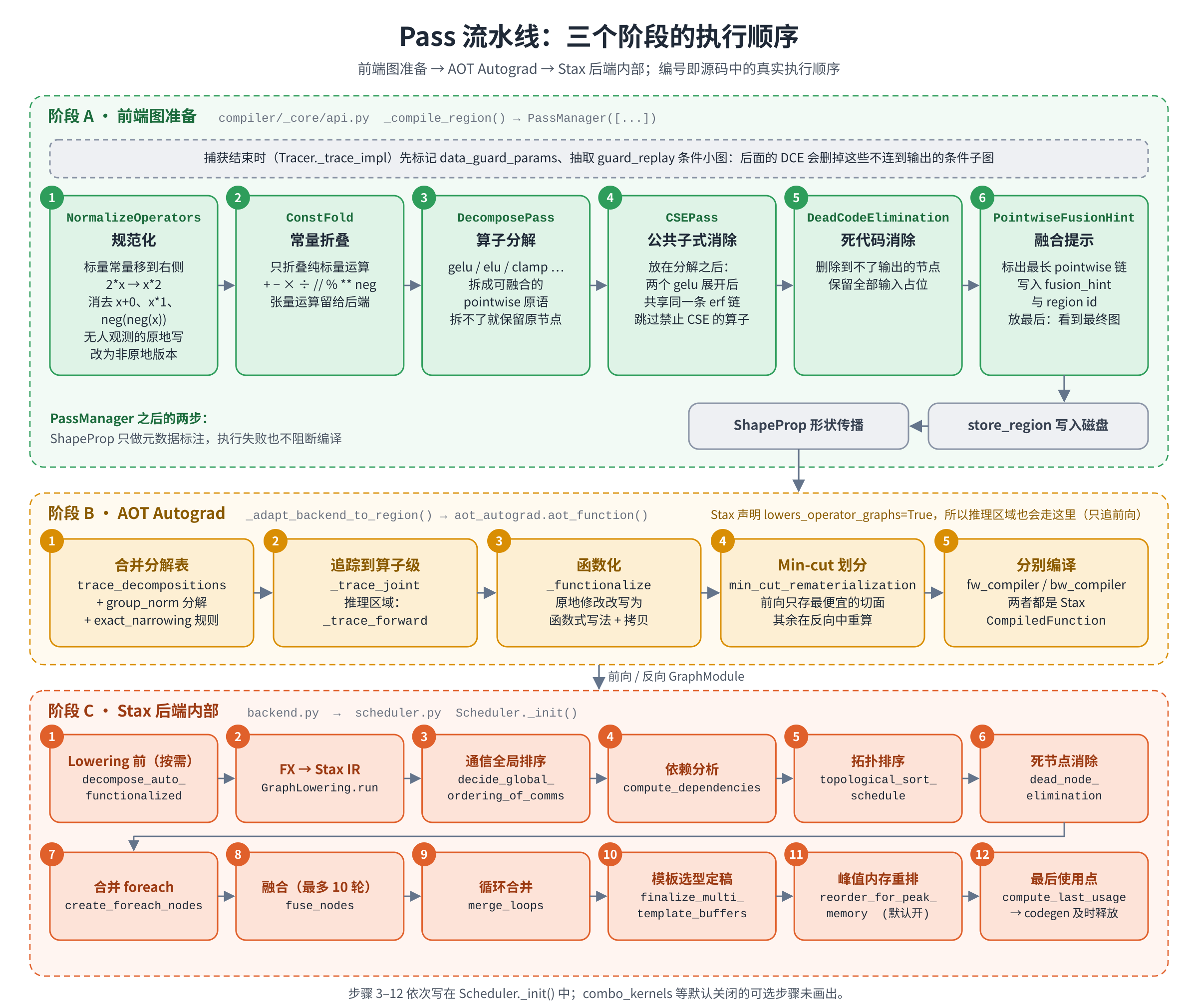
Figure 4.1 The order of the transformations in three stages. A is the front-end transformation of this section, B is the automatic differentiation layer of 第 Section 5, and C is a step inside the scheduler (第 Section 7).
Table of Contents | Next: Part Two Automatic Differentiation and Lowering